
The seemingly simple question, “what is the zero of g?”, transcends its pure mathematical definition to become a foundational concept in the vast and ever-evolving landscape of technology. Far from being a mere academic exercise, understanding and computing the “zero of g” — where ‘g’ represents a function, an algorithm’s output, or a system’s state — is critical for everything from designing sophisticated engineering systems and optimizing machine learning models to solving complex problems in scientific computing and artificial intelligence.
In essence, the “zero of g” refers to any input value (or set of values) for which the function ‘g’ yields an output of zero. While initially rooted in algebra and calculus, this principle has found profound practical applications across myriad technological domains, driving innovation and enabling functionalities that underpin our digital world. This article will delve into the multifaceted implications of finding the zero of ‘g’ within the tech sphere, exploring its fundamental concepts, its pivotal role in modern AI, its practical applications, and the inherent challenges in its computation.

The Fundamental Concept: Roots of Functions in Computing
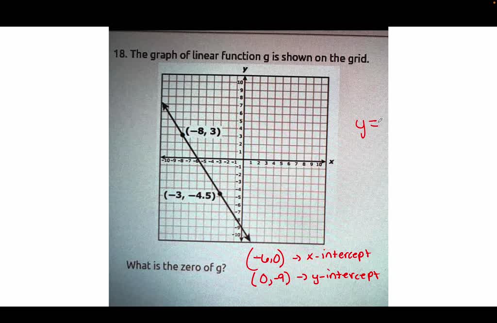
At its core, “the zero of g” is synonymous with finding the “roots” of a function. Mathematically, if you have a function g(x), its zero is any value x for which g(x) = 0. While this might bring back memories of high school algebra, its computational significance is far more reaching and complex.
Beyond Algebra: Why Zeros Matter in Software
In the realm of software and computational systems, the functions we deal with are often intricate, multi-variable, and non-linear, representing real-world physical phenomena, economic models, or complex data relationships. Finding the zeros of these functions is not just about solving an equation; it’s about identifying critical states, equilibrium points, optimal solutions, or specific conditions where a system achieves a desired outcome.
For instance, in engineering simulations, finding the zero of a force function might indicate a point of static equilibrium. In control systems, it could signify the point where a system achieves its target state with zero error. In scientific computing, solving for zeros of complex equations is fundamental to modeling everything from quantum mechanics to climate patterns. Software applications, therefore, rely heavily on robust numerical methods to approximate these zeros with high precision, as analytical solutions are often impossible or impractical for the complex functions encountered in practice.
Common Algorithms for Finding Zeros
Given the impossibility of finding analytical solutions for many functions, computational approaches rely on iterative numerical methods. These algorithms start with an initial guess and progressively refine it until a sufficiently accurate approximation of the zero is found.
-
Bisection Method: One of the simplest and most robust methods, the bisection method works by repeatedly halving the interval within which a zero is known to exist. It guarantees convergence if a zero is bracketed, but it can be relatively slow. Its reliability makes it a staple for ensuring solutions even with challenging functions.
-
Newton-Raphson Method: This method is significantly faster when it converges, leveraging the function’s derivative to project where the zero might lie. It iteratively refines an estimate using the tangent line at the current point. However, it requires the function to be differentiable and an initial guess close enough to the actual root, otherwise, it can diverge or converge to an unintended zero.
-
Secant Method: A powerful alternative to Newton-Raphson, the secant method doesn’t require the explicit computation of the derivative. Instead, it approximates the derivative using two previous points, making it suitable for functions where the derivative is difficult or impossible to calculate. It offers a good balance between speed and ease of implementation.
-
Brent’s Method: Often considered one of the best root-finding algorithms, Brent’s method is a hybrid approach combining the reliability of the bisection method with the speed of secant or inverse quadratic interpolation. It is robust, efficient, and widely used in numerical libraries due to its ability to handle a wide range of functions effectively.
The Zero of ‘g’ in Modern AI and Machine Learning
Perhaps nowhere is the concept of “the zero of g” more pervasive and critical than in the rapidly advancing fields of Artificial Intelligence (AI) and Machine Learning (ML). Here, ‘g’ often takes on new interpretations, representing error functions, gradients, or measures of system performance.
Gradient Descent and Optimization
In machine learning, the goal is often to train models to make accurate predictions or decisions. This is typically achieved by minimizing a “loss function” (or cost function), which quantifies the error between the model’s predictions and the actual values. The process of minimization is where the “zero of g” comes into play through techniques like Gradient Descent.
Here, ‘g’ is not the loss function itself, but rather the gradient of the loss function. The gradient points in the direction of the steepest ascent of the loss function. To minimize the loss, we need to move in the opposite direction of the gradient. The optimal parameters for a model are found when the gradient of the loss function is zero (or very close to zero), indicating that we’ve reached a local minimum or maximum (often a minimum for loss functions).
Think of it like being blindfolded on a mountain and trying to find the lowest point. You’d feel the slope (the gradient) and take steps in the direction that goes downhill. When you reach a point where there’s no more slope (the gradient is zero), you’ve found a local minimum. This iterative process of adjusting model parameters based on the gradient’s direction is the cornerstone of training neural networks, support vector machines, and many other ML algorithms.
Reinforcement Learning and Goal States
In Reinforcement Learning (RL), agents learn to make decisions by interacting with an environment to maximize a cumulative reward. While direct “zero of g” calculations might not always be explicit, the underlying principle is often present. For instance, in some RL problems, ‘g’ could represent the difference between the current state and a desired goal state. The agent’s objective is to reach a point where this difference ‘g’ becomes zero, signaling successful completion of a task.

Alternatively, ‘g’ could be a component of a value function or a policy gradient, where finding its zero (or a specific critical point) helps optimize the agent’s behavior to achieve maximal rewards or minimum costs, effectively navigating towards a “zero-cost” or “maximum-reward” state.
Practical Applications Across Technology
The utility of finding the zero of ‘g’ spans a diverse array of technological applications, proving its versatility and indispensable nature.
Engineering and Simulation
In virtually every branch of engineering, the ability to solve for zeros of functions is paramount.
- Circuit Design: Electrical engineers use Kirchhoff’s laws to model circuits. Solving these equations often involves finding points where current sums to zero or potential differences are zero, crucial for stable and efficient circuit operation.
- Structural Analysis: Civil and mechanical engineers analyze stress, strain, and deflection in structures. Finding points of zero stress or zero deflection helps identify critical load-bearing areas or points of equilibrium.
- Fluid Dynamics: Simulating fluid flow, whether for aircraft wings or weather patterns, involves complex partial differential equations. Numerical methods are used to find steady-state conditions where the rate of change of certain properties (like velocity or pressure) becomes zero.
- Robotics: For robot kinematics and dynamics, solving for joint angles or end-effector positions often translates to finding the zeros of geometric constraint equations, ensuring the robot reaches a desired target with zero positional error.
Data Science and Analytics
The field of data science heavily relies on statistical modeling and optimization, making zero-finding a key technique.
- Regression Analysis: When performing linear or non-linear regression, the goal is to find parameters that minimize the sum of squared residuals (the differences between observed and predicted values). This is essentially finding the zero of the derivative of the sum of squares function, optimizing the model’s fit to the data.
- Curve Fitting: Fitting complex curves to data points also involves minimizing an error function. The parameters of the curve are adjusted until the error function approaches zero, indicating the best possible fit.
- Statistical Inference: Many statistical tests and parameter estimations involve solving equations where a likelihood function’s derivative is set to zero to find maximum likelihood estimates.
Game Development and Robotics
Even in creative and dynamic fields like game development and robotics, the concept is fundamental.
- Game Physics Engines: Collision detection and resolution in games often involve calculating the point of zero overlap between objects to prevent unnatural interpenetration, or determining the forces needed to bring relative velocity to zero after impact.
- Pathfinding: In AI for games or robotics, an agent navigating to a target often employs algorithms that iteratively reduce a ‘distance to target’ function ‘g’ until it reaches zero, signifying the goal has been achieved.
- Control Systems: For robotic arms or autonomous vehicles, control algorithms continuously adjust inputs to minimize errors, effectively driving an error function ‘g’ to zero to maintain desired trajectories or positions.
Challenges and Considerations When Seeking the Zero of g
While immensely powerful, the computational search for the zero of ‘g’ is not without its complexities and challenges.
Multiple Zeros and Local Minima
Many functions, especially complex ones encountered in AI and engineering, can have multiple zeros or, in optimization contexts, multiple local minima. An iterative algorithm might converge to any one of these depending on the initial guess. For global optimization, where the absolute minimum or all zeros are desired, more sophisticated techniques like global search algorithms or multi-start strategies are required. Understanding the landscape of ‘g’ is crucial to ensure the algorithm finds the desired zero, not just any zero.
Computational Cost and Precision
Iterative numerical methods are, by nature, computationally intensive. Each iteration involves function evaluations, and sometimes derivative calculations, which can be costly for complex functions. There’s a constant trade-off between the desired precision of the zero and the computational resources (time and processing power) available. For real-time systems, approximate solutions obtained quickly might be preferable to perfectly accurate ones that take too long. Furthermore, floating-point arithmetic in computers introduces precision limitations, meaning a perfect zero (exactly 0.0) is rarely achieved; instead, solutions within a very small tolerance are accepted.
Non-Smooth Functions and Non-Existence of Zeros
Not all functions encountered in computational problems are well-behaved. Some might be non-differentiable, discontinuous, or even lack a true zero within a reasonable domain. For such functions, standard root-finding algorithms may fail or provide misleading results. In these cases, alternative approaches might be necessary, such as approximating the function with a smoother one, searching for points where the function’s value is minimized (even if not zero), or employing specialized robust optimizers designed for non-smooth landscapes. Additionally, some problems might not have a solution where ‘g’ is exactly zero, in which case the goal shifts to finding the point where ‘g’ is closest to zero.
Conclusion
The question, “what is the zero of g?”, serves as a gateway to understanding some of the most fundamental computational challenges and solutions across the technology spectrum. From the foundational numerical methods used to solve scientific equations to the intricate optimization algorithms powering modern artificial intelligence, the pursuit of the “zero of g” is an indispensable driver of progress. Whether it’s finding equilibrium in an engineering design, minimizing error in a machine learning model, or guiding a robot to its target, the ability to pinpoint these critical points allows systems to operate efficiently, intelligently, and effectively. As technology continues to advance, the sophistication and importance of accurately and efficiently finding the zero of ‘g’ will only continue to grow, solidifying its status as a cornerstone of digital innovation.
aViewFromTheCave is a participant in the Amazon Services LLC Associates Program, an affiliate advertising program designed to provide a means for sites to earn advertising fees by advertising and linking to Amazon.com. Amazon, the Amazon logo, AmazonSupply, and the AmazonSupply logo are trademarks of Amazon.com, Inc. or its affiliates. As an Amazon Associate we earn affiliate commissions from qualifying purchases.