What is an AVL Tree? Understanding the Foundations of Self-Balancing Data Structures

In the vast and intricate world of computer science, efficient data management is paramount. Whether you’re building a massive database, designing a lightning-fast search engine, or developing a complex operating system, the way data is stored, retrieved, and manipulated can significantly impact performance. At the heart of many high-performance systems lies a sophisticated data structure known as the AVL tree.

Named after its inventors, Georgy Adelson-Velsky and Evgenii Landis, who introduced it in 1962, an AVL tree stands as a testament to elegant algorithmic design. It is a self-balancing binary search tree (BST), a crucial distinction that elevates it beyond the limitations of a basic BST. While traditional BSTs offer average-case logarithmic time complexity for operations like search, insertion, and deletion, their worst-case performance can degrade to linear time if the tree becomes “skewed” or unbalanced. The AVL tree meticulously avoids this pitfall, guaranteeing logarithmic time complexity in all scenarios by employing a clever mechanism of rotations to maintain a strict balance. This article will delve into the core concepts, mechanisms, and importance of AVL trees, revealing why they remain a cornerstone of efficient data management in technology.

Table of Contents

The Core Concept: A Self-Balancing Binary Search Tree

To truly appreciate the genius of an AVL tree, one must first understand the fundamental challenges posed by its predecessor: the simple Binary Search Tree (BST).

Revisiting Binary Search Trees (BSTs): The Problem of Skewness

A Binary Search Tree is a hierarchical data structure where each node has at most two children, referred to as the left child and the right child. The defining characteristic of a BST is its ordering property: for any given node, all values in its left subtree are less than the node’s value, and all values in its right subtree are greater. This property makes searching incredibly efficient. If the tree is well-balanced, finding an element takes O(log n) time, where n is the number of nodes.

However, the efficiency of a BST hinges entirely on its balance. If elements are inserted in a sorted (or nearly sorted) order, the tree can degenerate into a linked list. Imagine inserting 1, 2, 3, 4, 5 into an empty BST. Node 1 would be the root, 2 its right child, 3 its right child, and so on. The tree would become a long, skinny chain. In such a “skewed” tree, searching for the last element would require traversing every node, leading to O(n) time complexity, no better than a linear scan through an array. This worst-case scenario undermines the primary advantage of a BST.

The “Self-Balancing” Mechanism: Maintaining Height Balance

This is where the “self-balancing” aspect of an AVL tree comes into play. An AVL tree is not merely a BST; it’s a height-balanced BST. The key constraint that defines an AVL tree is that for every node, the heights of its left and right subtrees must differ by at most 1. This seemingly simple rule has profound implications for the tree’s structure and performance. By enforcing this strict balance, an AVL tree ensures that its height always remains logarithmic with respect to the number of nodes. This logarithmic height, in turn, guarantees O(log n) time complexity for search, insertion, and deletion operations, even in the worst-case scenario.

Balance Factor: The Metric for Equilibrium

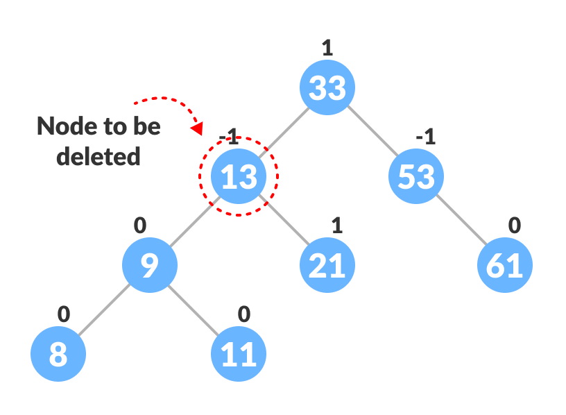
To maintain this balance criterion, each node in an AVL tree typically stores an additional piece of information: its balance factor. The balance factor of a node is calculated as the height of its right subtree minus the height of its left subtree. According to the AVL property, a node’s balance factor can only be -1, 0, or 1.

-1: The left subtree is one level taller than the right subtree.
0: Both subtrees have the same height.
1: The right subtree is one level taller than the left subtree.

If, after an insertion or deletion operation, any node’s balance factor deviates from this range (i.e., becomes -2 or 2), the tree is considered out of balance at that node. This imbalance triggers a series of rebalancing operations, primarily through rotations, to restore the AVL property.

How AVL Trees Maintain Balance: Rotations Explained

The magic behind an AVL tree’s self-balancing capability lies in a set of structural transformations called rotations. These operations rearrange nodes in a localized manner to restore the balance factor constraint without violating the fundamental BST ordering property.

Understanding Node Rotations: Left, Right, Left-Right, Right-Left

When an insertion or deletion causes a node to become unbalanced (balance factor -2 or 2), a rotation (or a pair of rotations) is performed at the lowest unbalanced ancestor node. There are four fundamental types of rotations, categorized into single rotations and double rotations.

Single Rotations: Left Rotation and Right Rotation

Single rotations are used when an imbalance occurs in a “straight line” or “zig-zig” configuration.

Left Rotation: This occurs when a node becomes right-heavy (balance factor 2) because a new node was inserted into its right child’s right subtree. To rebalance, the right child becomes the new parent, the original parent becomes its left child, and the original right child’s left subtree (if any) becomes the new left child’s right subtree. This effectively “rotates” the right child upwards and the parent downwards and to the left.
- Example: If a node A has B as its right child, and B has C as its right child, and C causes A to become unbalanced, a left rotation at A would make B the new root of this subtree, with A as its left child and C as its right child.
Right Rotation: This is the mirror image of a left rotation. It occurs when a node becomes left-heavy (balance factor -2) because a new node was inserted into its left child’s left subtree. The left child becomes the new parent, the original parent becomes its right child, and the original left child’s right subtree (if any) becomes the new right child’s left subtree.
- Example: If a node A has B as its left child, and B has C as its left child, and C causes A to become unbalanced, a right rotation at A would make B the new root of this subtree, with C as its left child and A as its right child.

Double Rotations: Left-Right Rotation and Right-Left Rotation

Double rotations are required when an imbalance occurs in a “zig-zag” configuration, meaning the new node was inserted into an inner subtree.

Left-Right Rotation: This is needed when a node A is left-heavy (balance factor -2) because an insertion occurred in the right subtree of its left child (B). A single right rotation at A would not fix the balance. Instead, a left rotation is first performed on B (the left child of A), then a right rotation is performed on A. This effectively brings the problematic grandchild node up to become the new parent.
Right-Left Rotation: This is the mirror image. It’s needed when a node A is right-heavy (balance factor 2) because an insertion occurred in the left subtree of its right child (B). A right rotation is first performed on B (the right child of A), then a left rotation is performed on A.

The Rotation Process: When and How They Occur

Rotations are always performed from the bottom up. After an insertion, the algorithm traverses back up the tree from the newly inserted node to the root. At each node along this path, it updates the height and balance factor. If a node’s balance factor becomes -2 or 2, the appropriate rotation (or sequence of rotations) is performed to restore balance. This localized rebalancing ensures that the entire tree remains balanced with minimal structural changes.

Operations on an AVL Tree: Beyond Simple BST Logic

While an AVL tree fundamentally adheres to the BST property, its self-balancing nature introduces additional steps for insertion and deletion compared to a basic BST. Searching, however, benefits directly from the guaranteed balance.

Insertion: Identifying Imbalance and Applying Rotations

The insertion process in an AVL tree begins much like a standard BST insertion:

Search for insertion point: Traverse the tree to find the correct leaf node position where the new element should be inserted, maintaining the BST property.
Insert the node: Add the new node as a child of the identified leaf.
Update heights and balance factors: Travel back up the path from the inserted node to the root. For each node encountered, recompute its height and balance factor.
Perform rotations (if necessary): If, during the upward traversal, a node is found to have a balance factor of -2 or 2, perform the necessary single or double rotation(s) at that node to restore balance. This rebalancing might propagate upwards, affecting ancestor nodes, but typically a single set of rotations fixes the imbalance in the affected subtree, and the balance property is restored for the entire path above it.

Deletion: A More Complex Balancing Act

Deletion in an AVL tree is more intricate than insertion because removing a node can potentially cause imbalances in a broader range of ancestor nodes.

Search for the node to delete: Locate the node N that needs to be removed.
Perform standard BST deletion:
- If N is a leaf node, simply remove it.
- If N has one child, replace N with its child.
- If N has two children, find its in-order successor (the smallest node in its right subtree) or predecessor (the largest node in its left subtree), copy its value to N, and then recursively delete the successor/predecessor node.
Update heights and balance factors: After the actual removal (or replacement with successor/predecessor), traverse upwards from the parent of the actually deleted node (or the replaced successor/predecessor) all the way to the root.
Perform rotations (if necessary): At each node on this upward path, update its height and balance factor. If an imbalance (-2 or 2) is detected, perform the appropriate single or double rotation(s). Unlike insertion, where one rotation might suffice for the path, deletion might require multiple rotations up the path, as a rebalance at one level might cause a new imbalance further up.

Search: The Logarithmic Efficiency

Searching in an AVL tree is identical to searching in a regular BST. The key difference is the guaranteed performance. Because an AVL tree is always height-balanced, the search path will never exceed log n levels. This means that an AVL tree guarantees O(log n) time complexity for search operations, regardless of the order in which elements were inserted, making it a highly reliable choice for applications requiring predictable search performance.

Why AVL Trees Matter: Performance and Practical Applications

The AVL tree’s commitment to balance makes it a standout choice for certain technological applications, emphasizing its importance in scenarios where consistent performance is critical.

Guaranteed Logarithmic Time Complexity

The most significant advantage of an AVL tree is its strict guarantee of O(log n) time complexity for all fundamental operations: search, insertion, and deletion. This predictability is invaluable in real-time systems, mission-critical applications, and scenarios where worst-case performance must be tightly controlled. Unlike a basic BST, whose performance can degrade severely, an AVL tree provides a consistent, efficient experience. This guarantee stems directly from its height-balancing property, which ensures the tree’s height never becomes disproportionately large.

Comparison with Other Self-Balancing Trees (e.g., Red-Black Trees)

While AVL trees were pioneering, other self-balancing BSTs have emerged. Red-Black trees, for instance, are another popular type.

AVL Trees vs. Red-Black Trees: Both guarantee O(log n) performance. However, AVL trees are more strictly balanced than Red-Black trees. The height difference in an AVL tree is at most 1, whereas in a Red-Black tree, it can be up to twice the minimum possible height. This tighter balance means AVL trees generally offer faster search times because the average path length to any node is shorter.
Trade-offs: The trade-off for AVL’s stricter balance is that insertions and deletions might require more rotations (or more complex rotation sequences) to maintain that balance compared to Red-Black trees. Red-Black trees often have fewer rotations on average, making them slightly faster for write-heavy (insertion/deletion intensive) workloads, while AVL trees shine in read-heavy (search intensive) scenarios. Red-Black trees are also generally easier to implement due to slightly simpler rebalancing rules. Many standard library implementations (like std::map in C++ or TreeMap in Java) use Red-Black trees.

Real-World Use Cases: Databases, File Systems, Network Routers

Despite the existence of other self-balancing trees, AVL trees remain a fundamental concept and find practical utility:

Databases: Indexing is a critical component of database management systems. AVL trees can be used to implement indexes, allowing for rapid retrieval of records based on key values. Their guaranteed O(log n) search time ensures consistent query performance.
File Systems: Some file systems use AVL trees or similar structures for managing file metadata, directory structures, or inode tables, enabling fast lookups for files and directories.
Network Routers: In high-speed network routers, fast lookup tables are essential for forwarding packets. AVL trees can be employed to efficiently store and search routing tables or IP addresses.
In-memory Data Management: For applications that require dynamic, ordered data storage with predictable performance, AVL trees are an excellent choice for in-memory data structures, such as symbol tables in compilers or dictionaries.

Implementing AVL Trees: Key Considerations

Implementing an AVL tree requires careful attention to detail, especially in managing node heights and performing rotations.

Data Structure Representation

Each node in an AVL tree typically stores:

key: The value stored in the node.
value: (Optional) The associated data for the key.
left_child_pointer: Pointer to the left child node.
right_child_pointer: Pointer to the right child node.
height: The height of the node’s subtree (distance to the deepest leaf). This is crucial for calculating the balance factor.

The height field is continuously updated after every insertion or deletion, and the balance factor is derived from the heights of the children.

Algorithmic Complexity of Operations

Search: O(log n) – Due to the guaranteed balanced height.
Insertion: O(log n) – Involves a log n traversal to find the insertion point, followed by at most one single or double rotation, and log n height updates.
Deletion: O(log n) – Involves a log n traversal to find the node, potentially a log n traversal to find a successor, and then potentially log n rotations and height updates up the path to the root.

All operations maintain their logarithmic complexity, which is the primary strength of AVL trees.

Conclusion

The AVL tree is more than just a historical artifact in computer science; it remains a powerful and foundational concept for understanding efficient data management. By rigorously enforcing a height-balance property through a series of elegant rotations, AVL trees overcome the performance pitfalls of degenerate binary search trees. They guarantee logarithmic time complexity for all core operations, making them an excellent choice for applications that demand consistent, predictable, and high-performance data access. While other self-balancing trees like Red-Black trees offer alternative trade-offs, the AVL tree’s conceptual elegance and strict balance criteria continue to make it a vital component in the toolkit of any technologist seeking to build robust and efficient systems. Understanding “what is an AVL tree” is to grasp a fundamental principle of how technology ensures fast and reliable data handling in a complex digital world.

aViewFromTheCave is a participant in the Amazon Services LLC Associates Program, an affiliate advertising program designed to provide a means for sites to earn advertising fees by advertising and linking to Amazon.com. Amazon, the Amazon logo, AmazonSupply, and the AmazonSupply logo are trademarks of Amazon.com, Inc. or its affiliates. As an Amazon Associate we earn affiliate commissions from qualifying purchases.