In the intricate world of finance, where every decision carries an element of uncertainty, understanding risk is paramount. Investors, financial analysts, and business leaders constantly seek robust tools to measure and interpret the potential variability of returns, market movements, or investment performance. Among the most fundamental and widely utilized statistical concepts for this purpose is the standard deviation. More specifically, delving into “two standard deviations” provides a profound insight into the probable range of outcomes, helping to delineate what is considered typical versus what might be an outlier in financial data.
This concept isn’t just academic; it’s a cornerstone of practical financial management, informing everything from individual stock analysis to sophisticated portfolio construction and macroeconomic forecasting. By grasping what two standard deviations represent, individuals and institutions can make more informed decisions, better manage expectations, and build resilience against the inherent volatility of financial markets. It offers a standardized way to quantify dispersion, allowing for meaningful comparisons and a clearer perspective on the risk-reward landscape. Let’s explore how this powerful statistical measure translates into actionable financial intelligence.
Understanding the Core Concept: Standard Deviation
Before we unpack the significance of “two standard deviations,” it’s crucial to first understand its foundational component: the standard deviation itself. At its heart, standard deviation is a measure of the amount of variation or dispersion of a set of values. A low standard deviation indicates that the values tend to be close to the mean (average) of the set, while a high standard deviation indicates that the values are spread out over a wider range.
The Basics of Data Spread
Imagine you have a series of monthly returns for an investment over a year. Some months it might gain 5%, others 2%, some might lose 1%, and so on. The mean return tells you the average performance, but it doesn’t tell you how volatile that performance was. Was it consistently close to the average, or were there wild swings? This is where standard deviation comes in. It quantifies the typical distance each data point is from the mean.
Mathematically, standard deviation is calculated as the square root of the variance, where variance is the average of the squared differences from the mean. While the calculation itself might seem intimidating to the uninitiated, the conceptual takeaway is simple: it’s a single number that tells you how “spread out” your data is. In finance, this “spread” is directly analogous to risk.
Why Standard Deviation Matters in Finance
In the realm of money and investing, standard deviation is almost universally adopted as the primary measure of an asset’s or portfolio’s historical volatility. When you hear that an investment is “risky,” it often implies that its past returns have shown a high standard deviation, meaning its returns have fluctuated significantly around its average. Conversely, a “safe” investment typically exhibits a low standard deviation, indicating more predictable and consistent returns.
For instance, comparing two investments that both have an average annual return of 10%: if Investment A has a standard deviation of 5% and Investment B has a standard deviation of 20%, Investment A is considered less risky because its returns are more consistently around the 10% average. Investment B, despite the same average return, has experienced much wider swings, implying a higher potential for both large gains and significant losses. This metric allows investors to objectively compare the risk profiles of different assets, a critical step in making informed allocation decisions.
The Power of Two Standard Deviations in Investment Analysis
While the standard deviation provides a crucial baseline for understanding volatility, looking at “two standard deviations” transforms this basic measure into a powerful predictive tool, especially when dealing with data that approximates a normal distribution.
Quantifying Risk and Volatility
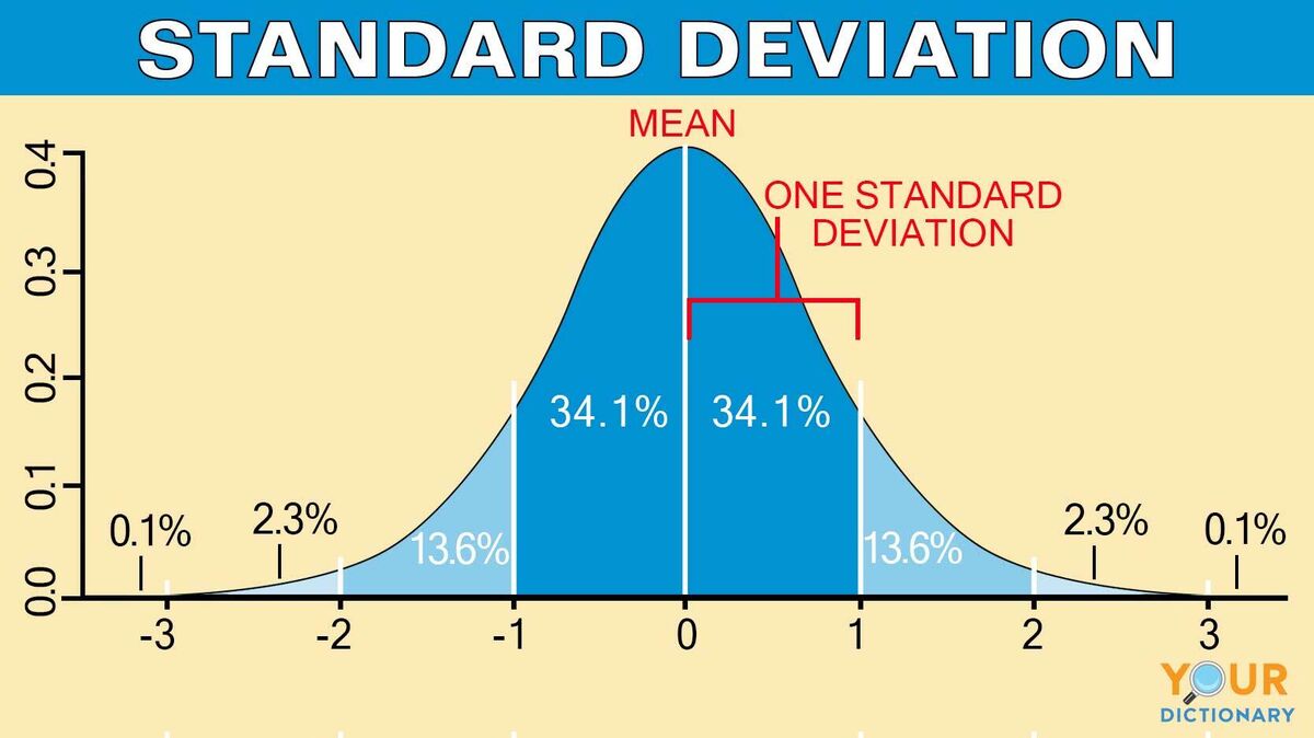
For many financial phenomena—such as daily stock price changes, investment returns over long periods, or even macroeconomic indicators—the data often follows a bell-shaped curve known as a normal distribution. In a normal distribution, specific percentages of the data fall within certain standard deviation ranges from the mean. This is where the renowned “68-95-99.7 rule” or “Empirical Rule” becomes incredibly valuable.
This rule states:
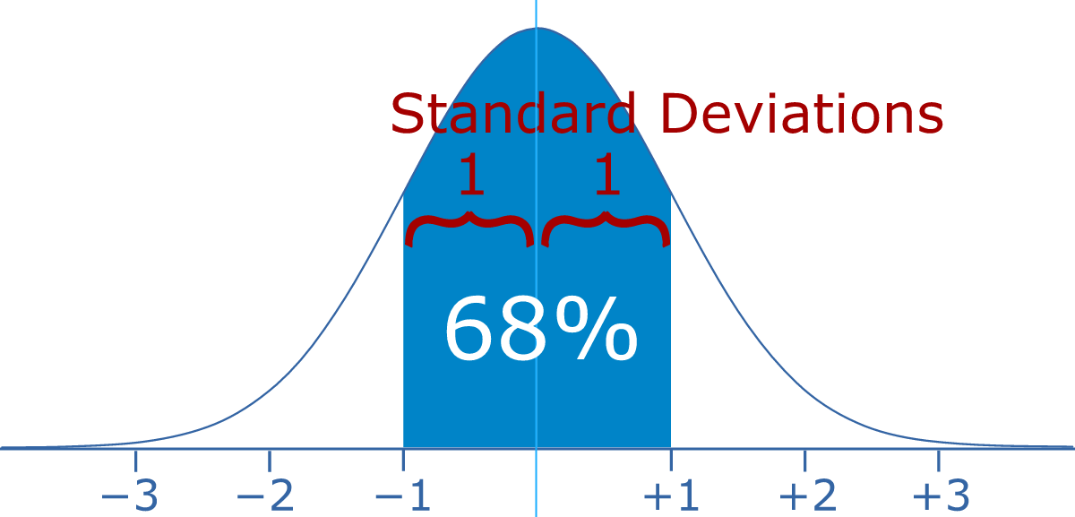
- Approximately 68% of data falls within one standard deviation of the mean.
- Approximately 95% of data falls within two standard deviations of the mean.
- Approximately 99.7% of data falls within three standard deviations of the mean.
When we talk about “two standard deviations,” we are essentially identifying a range around the average within which roughly 95% of all observed outcomes are expected to fall. This means that if an investment’s average annual return is 8% and its standard deviation is 5%, then there’s approximately a 95% chance that its annual return will fall between -2% (8% – 25%) and 18% (8% + 25%). This range offers a much more nuanced understanding of potential performance than just the average return alone.
Identifying Expected Ranges and Outliers
The significance of the 95% confidence interval offered by two standard deviations cannot be overstated in finance. It allows investors to:
- Set Realistic Expectations: By understanding this range, investors can temper overly optimistic projections and prepare for potential downturns. It clarifies that while the average return might be attractive, there’s a significant likelihood of outcomes falling within a wider, potentially less favorable, spectrum.
- Identify Outliers and Black Swan Events: When an actual return or market movement falls outside the two-standard-deviation range, it’s considered a statistically significant event—an outlier. While not impossible, such events are less common (occurring approximately 5% of the time). Events falling outside three standard deviations are even rarer (0.3% of the time) and are often termed “black swan” events or extreme market shocks, which can have profound implications for unprepared portfolios. This framework helps differentiate between normal market fluctuations and genuinely unusual occurrences that might warrant a re-evaluation of strategies.
- Assess Value at Risk (VaR): For financial institutions and sophisticated investors, the two-standard-deviation concept is directly applied in calculating Value at Risk (VaR). VaR estimates the maximum expected loss over a given period at a specified confidence level, typically 95% or 99%. A 95% VaR, for instance, tells you the maximum loss you can expect to incur on 95% of trading days or periods, directly leveraging the understanding of two standard deviations from the mean.
Practical Applications in Personal Finance and Investing
The theoretical understanding of two standard deviations truly shines when applied to practical financial scenarios, offering robust insights for both individual investors and professional financial managers.
Assessing Individual Investments (Stocks, Bonds, Funds)
When evaluating individual assets like stocks, bonds, or mutual funds, standard deviation (and by extension, two standard deviations) is a critical component of risk assessment. A high standard deviation for a stock indicates that its price has historically been very volatile, prone to large swings. This might appeal to risk-tolerant investors seeking higher potential returns, but it also signals a greater chance of significant losses. Conversely, a bond fund with a low standard deviation suggests more stable returns and lower risk, appealing to conservative investors.
Financial tools and platforms often display an investment’s historical standard deviation. Investors can use this to compare the risk level of various options. For example, if comparing two growth funds, one with a standard deviation of 15% and another with 25%, the latter is inherently riskier, implying a wider potential range of returns (two standard deviations would encompass a 30% and 50% range around the mean, respectively). This allows for a more objective, data-driven comparison of risk profiles beyond just anecdotal perceptions.
Building and Managing a Diversified Portfolio
Perhaps one of the most powerful applications of standard deviation in finance is in portfolio management. Modern Portfolio Theory (MPT) emphasizes diversification as a means to optimize risk and return. By combining assets whose returns are not perfectly correlated, investors can reduce the overall standard deviation (risk) of their portfolio without necessarily sacrificing returns.
Financial advisors use standard deviation to construct portfolios tailored to a client’s risk tolerance. A conservative investor’s portfolio will aim for a lower overall standard deviation, achieved by including a higher proportion of less volatile assets like bonds or stable dividend stocks. An aggressive investor might tolerate a higher portfolio standard deviation in pursuit of greater returns, allocating more to growth stocks or emerging markets. Understanding the probable range of portfolio returns (e.g., within two standard deviations) helps both the advisor and client set realistic expectations and maintain discipline during market fluctuations. It provides a data-backed estimate of the worst-case (and best-case) scenarios over a typical investment horizon.
Gauging Market Sentiment and Economic Health
Beyond individual investments, standard deviation can also be applied to broader market indices like the S&P 500 or NASDAQ. A period of unusually high standard deviation for an index suggests increased market volatility and uncertainty, often coinciding with economic downturns, geopolitical events, or significant policy changes. Conversely, a low standard deviation indicates a period of relative calm and stability.
Financial analysts monitor these shifts closely. For instance, if the average daily movement of a market index is 0.5% with a standard deviation of 1%, a day where the market moves 2.5% in either direction would be considered outside two standard deviations (0.5% +/- 2*1% = -1.5% to 2.5%). Such a large move would signal a statistically significant event, prompting deeper investigation into its causes and potential implications for future market direction and economic health. It helps distinguish between routine market noise and substantial shifts in investor sentiment or underlying economic conditions.
Navigating Risk: Limitations and Strategic Considerations
While the concept of two standard deviations is invaluable, it’s not a perfect crystal ball. Its utility is greatest when understood within its limitations and integrated with other financial metrics and considerations.
Beyond Normal Distributions: Skewness and Kurtosis
The 68-95-99.7 rule, and thus the precision of the two-standard-deviation range, relies on the assumption that the data follows a normal distribution. However, financial returns often exhibit “fat tails” (more frequent extreme events) and skewness (asymmetrical distribution), meaning they are not perfectly normal. Markets can crash much faster than they rise, leading to negative skewness, and extreme price movements (both up and down) can be more common than a normal distribution would predict, reflecting higher kurtosis.
When distributions are not normal, relying solely on standard deviation can underestimate true risk. A portfolio might experience losses outside the two-standard-deviation range more frequently than the theoretical 5% suggests. Therefore, sophisticated analyses also consider metrics like skewness (to assess the asymmetry of returns) and kurtosis (to measure the “tailedness” of the distribution) to provide a more complete picture of risk. For most retail investors, however, standard deviation still provides a robust and accessible starting point.
The Role of Time Horizons and Investment Goals
The interpretation of standard deviation, and particularly the implications of two standard deviations, must always be contextualized by an investor’s time horizon and financial goals. For a short-term trader, a high standard deviation implies significant daily price swings, which could be opportunities or major risks. For a long-term investor with a 20-year horizon, short-term volatility (even outside two standard deviations) might be less concerning, as the focus shifts to compounding returns over time.
Similarly, an investor saving for retirement will view risk differently than someone saving for a down payment in two years. The same two-standard-deviation range that signals potential short-term losses for the latter might be seen as merely part of the journey for the former. Understanding your personal risk tolerance and time horizon is crucial to effectively apply statistical insights to your unique financial situation.
Integrating Standard Deviation with Other Financial Metrics
Standard deviation is a powerful standalone metric, but it gains even more utility when combined with other financial ratios and tools. For instance, the Sharpe Ratio uses standard deviation to measure risk-adjusted return, telling you how much excess return you’re getting per unit of risk. The Treynor Ratio similarly assesses returns relative to systematic risk.
Furthermore, qualitative factors like market sentiment, economic forecasts, regulatory changes, and company-specific news must always complement quantitative analysis. No statistical model can perfectly predict the future, and human behavior, irrational exuberance, and panic play significant roles in market movements, sometimes driving events far beyond any statistical prediction. Therefore, standard deviation serves as an excellent compass, but not the entire map.

Empowering Your Financial Decisions with Statistical Insight
In conclusion, understanding “what is two standard deviations” provides a critical lens through which to view the inherent uncertainty of the financial world. It transcends mere academic curiosity, serving as a practical, actionable framework for quantifying risk, setting realistic expectations, and identifying significant market events.
By grasping that roughly 95% of expected outcomes lie within this range, investors gain a powerful tool for comparing assets, constructing resilient portfolios, and interpreting market volatility. While acknowledging its statistical assumptions and limitations, integrating this knowledge empowers individuals and businesses to navigate the complex currents of financial markets with greater confidence and foresight. It allows for a more disciplined approach to investing, shifting the focus from speculative guesses to informed decisions grounded in statistical probability. In a financial landscape that is constantly evolving, such foundational insights remain invaluable for achieving long-term success and financial well-being.
aViewFromTheCave is a participant in the Amazon Services LLC Associates Program, an affiliate advertising program designed to provide a means for sites to earn advertising fees by advertising and linking to Amazon.com. Amazon, the Amazon logo, AmazonSupply, and the AmazonSupply logo are trademarks of Amazon.com, Inc. or its affiliates. As an Amazon Associate we earn affiliate commissions from qualifying purchases.