The 5-number summary is a fundamental statistical tool used to describe the distribution of a dataset concisely. It provides a quick overview of the central tendency, spread, and potential outliers of a set of data points. In essence, it’s a snapshot that reveals the shape of your data without needing to examine every single value. For anyone working with data, from students learning statistics to professionals analyzing market trends or financial performance, understanding the 5-number summary is crucial. It forms the bedrock for more complex statistical analyses and visualizations like box plots.
The Core Components of a 5-Number Summary
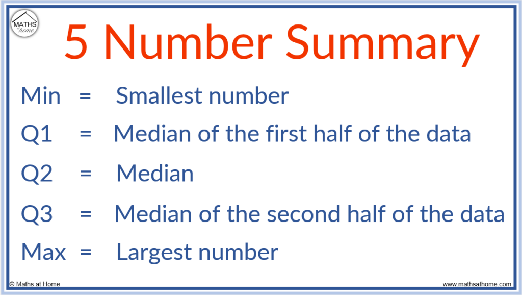
A 5-number summary is precisely what its name suggests: a set of five key statistical values that encapsulate the essential characteristics of a dataset. These five numbers are: the minimum, the first quartile (Q1), the median (Q2), the third quartile (Q3), and the maximum. Each of these values provides a unique piece of information about the data’s distribution. Let’s delve into each component in detail.

Minimum
The minimum value is the smallest data point in the dataset. It represents the absolute lowest observed value. Identifying the minimum is straightforward; it’s simply the lowest number in your ordered list of data. While seemingly simple, the minimum can be a crucial indicator, especially when assessing risk or identifying potential errors in data collection. For instance, in a dataset of product prices, the minimum would represent the cheapest item available. In a financial context, it might signify the lowest point a stock reached over a given period.
Maximum
Conversely, the maximum value is the largest data point in the dataset. It represents the absolute highest observed value. Similar to the minimum, finding the maximum involves identifying the largest number in your ordered data. The maximum is equally important as the minimum. In a sales dataset, it would show the highest single sale. In performance metrics, it could highlight the peak achievement. Both minimum and maximum values are critical for understanding the full range of variability within a dataset.
Median (Q2)
The median is the middle value of a dataset when it is ordered from least to greatest. It’s the point that divides the dataset into two equal halves, meaning 50% of the data points are below the median, and 50% are above it. To find the median:
- For an odd number of data points: Arrange the data in ascending order. The median is the middle number. For example, in the dataset {2, 5, 7, 9, 11}, the median is 7.
- For an even number of data points: Arrange the data in ascending order. The median is the average of the two middle numbers. For example, in the dataset {3, 6, 8, 10, 12, 15}, the two middle numbers are 8 and 10. The median is (8 + 10) / 2 = 9.
The median is a robust measure of central tendency because it is not affected by extreme outliers. This makes it particularly useful for skewed distributions where a few very high or very low values could significantly distort the mean (average).
Quartiles (Q1 and Q3)
Quartiles divide an ordered dataset into four equal parts.
First Quartile (Q1)
The first quartile, often denoted as Q1, is the median of the lower half of the dataset. This means it’s the value below which 25% of the data points lie. To calculate Q1:
- Order your dataset from least to greatest.
- Find the median of the entire dataset.
- Consider only the data points that are below the median.
- The median of this lower half is Q1.
Example: For the dataset {2, 5, 7, 9, 11, 13, 15}, the median is 9. The lower half is {2, 5, 7}. The median of this lower half (Q1) is 5.
Third Quartile (Q3)
The third quartile, denoted as Q3, is the median of the upper half of the dataset. This means it’s the value below which 75% of the data points lie (or above which 25% of the data points lie). To calculate Q3:
- Order your dataset from least to greatest.
- Find the median of the entire dataset.
- Consider only the data points that are above the median.
- The median of this upper half is Q3.
Example: For the dataset {2, 5, 7, 9, 11, 13, 15}, the median is 9. The upper half is {11, 13, 15}. The median of this upper half (Q3) is 13.
The quartiles, along with the median, provide a clearer picture of the data’s spread and concentration. They help us understand how the data is distributed within the lower and upper portions of the range.
Beyond the Numbers: What the 5-Number Summary Reveals
While the five individual numbers are important, their true power lies in how they work together to reveal the underlying structure and characteristics of the data. The 5-number summary provides insights into the data’s range, spread, and potential skewness, making it an invaluable tool for initial data exploration.
Range and Interquartile Range (IQR)
Two key measures of spread can be derived directly from the 5-number summary: the range and the Interquartile Range (IQR).
Range
The range is the simplest measure of spread and is calculated by subtracting the minimum value from the maximum value:
Range = Maximum – Minimum
The range gives us the total span of the data. A large range indicates that the data points are widely dispersed, while a small range suggests that the data points are clustered closely together. However, the range is highly sensitive to outliers. A single extremely high or low value can inflate the range significantly, potentially misrepresenting the typical spread of the majority of the data.
Interquartile Range (IQR)
The Interquartile Range (IQR) is a more robust measure of spread because it focuses on the middle 50% of the data. It is calculated by subtracting the first quartile (Q1) from the third quartile (Q3):
IQR = Q3 – Q1
The IQR represents the spread of the central portion of the data. It is less affected by extreme values than the range, making it a more reliable indicator of the typical variability within a dataset, especially when outliers are present. A larger IQR indicates greater variability in the middle 50% of the data, while a smaller IQR suggests that the middle 50% of the data is more tightly clustered.
Skewness and Outlier Detection
The relationships between the minimum, maximum, median, and quartiles can also provide clues about the skewness of the data distribution and help identify potential outliers.
Understanding Skewness
Skewness refers to the asymmetry of a probability distribution.
- Symmetric Distribution: If the data is perfectly symmetric, the median will be exactly in the middle of the range, and the distance from the median to Q1 will be roughly equal to the distance from the median to Q3. The mean and median will be very close.
- Right (Positive) Skew: If the data is skewed to the right, it means there’s a longer tail on the right side of the distribution, with more data points clustered on the lower end. In this case, the median will be closer to Q1, and the distance from the median to Q3 will be greater than the distance from the median to Q1. The maximum value will also be further from the median than the minimum value. The mean will typically be greater than the median.
- Left (Negative) Skew: If the data is skewed to the left, it means there’s a longer tail on the left side of the distribution, with more data points clustered on the higher end. Here, the median will be closer to Q3, and the distance from the median to Q1 will be greater than the distance from the median to Q3. The minimum value will be further from the median than the maximum value. The mean will typically be less than the median.
Identifying Potential Outliers
Outliers are data points that significantly differ from other observations in a dataset. The 5-number summary, particularly through the IQR, helps in identifying potential outliers. A common rule of thumb for identifying outliers is:
- Lower Outliers: Any data point that is less than Q1 – 1.5 * IQR is considered a potential outlier.
- Upper Outliers: Any data point that is greater than Q3 + 1.5 * IQR is considered a potential outlier.
These boundaries are often referred to as the “fences” of a box plot. Data points falling outside these fences are flagged for further investigation. It’s important to note that “potential outlier” means it warrants a closer look; it doesn’t automatically mean the data point is erroneous or should be removed. Context is crucial in determining if an outlier is valid or requires correction.
Applications of the 5-Number Summary
The 5-number summary is a versatile statistical concept with broad applications across various fields, particularly in data analysis and visualization. Its simplicity and effectiveness make it a go-to tool for quickly understanding data characteristics.
Data Visualization: The Box Plot
One of the most common and insightful applications of the 5-number summary is in the creation of box plots (also known as box-and-whisker plots). A box plot visually represents the 5-number summary of a dataset.
- The box itself spans from Q1 to Q3, with a line inside marking the median. The length of the box represents the IQR.
- The whiskers extend from the box to the minimum and maximum values (or to the furthest data points within the 1.5 * IQR rule, with individual points plotted beyond that as outliers).
Box plots are excellent for:
- Comparing distributions: Multiple box plots can be placed side-by-side to compare the spread, central tendency, and skewness of different datasets.
- Identifying outliers: Outliers are typically plotted as individual points beyond the whiskers.
- Grasping data spread quickly: The visual representation provides an immediate understanding of the data’s variability.
Descriptive Statistics and Reporting
In any field that involves data analysis, from academic research to business intelligence, the 5-number summary serves as a fundamental component of descriptive statistics. When presenting data, providing the minimum, Q1, median, Q3, and maximum alongside measures like the mean and standard deviation offers a comprehensive overview. This is especially valuable for:
- Initial Data Exploration: Before diving into complex modeling, understanding the basic characteristics through the 5-number summary helps identify patterns and potential issues.
- Executive Summaries: For stakeholders who need a quick grasp of data performance without delving into technical details, the 5-number summary provides a clear and concise picture.
- Benchmarking: Comparing the 5-number summary of a current dataset against historical data or industry benchmarks can reveal performance trends and areas for improvement.

Risk Assessment and Financial Analysis
In finance, the 5-number summary is invaluable for understanding the risk and return profile of investments.
- Stock Performance: When analyzing historical stock prices, the 5-number summary can show the lowest price (minimum), highest price (maximum), and the price ranges for the central 50% of trading days (IQR). The median indicates the typical daily trading price. This helps investors understand the volatility and potential upside/downside of an asset.
- Portfolio Analysis: For a portfolio of assets, calculating the 5-number summary for the returns of each asset can inform diversification strategies and risk management.
- Budgeting and Forecasting: In business finance, analyzing expense data using a 5-number summary can reveal the typical spending patterns, extreme expenditures (maximum), and minimum costs, aiding in more accurate budgeting and financial planning.
The 5-number summary, therefore, is not just a set of numbers; it’s a powerful analytical lens that simplifies complex data into understandable and actionable insights. Its ability to capture the essence of a dataset’s distribution makes it an indispensable tool in the data analyst’s toolkit.
aViewFromTheCave is a participant in the Amazon Services LLC Associates Program, an affiliate advertising program designed to provide a means for sites to earn advertising fees by advertising and linking to Amazon.com. Amazon, the Amazon logo, AmazonSupply, and the AmazonSupply logo are trademarks of Amazon.com, Inc. or its affiliates. As an Amazon Associate we earn affiliate commissions from qualifying purchases.