
In an increasingly data-driven and complex world, understanding and predicting outcomes under conditions of uncertainty is paramount. Whether designing a new software system, optimizing an AI algorithm, or evaluating the resilience of a network, developers and engineers constantly grapple with variables that are inherently random or unpredictable. This is where Monte Carlo analysis, a powerful computational technique, offers a robust solution, providing a framework to model and analyze systems where randomness plays a significant role. It transforms complex, probabilistic problems into a series of simulations, yielding a spectrum of possible outcomes and their associated probabilities.

The Core Concept: Simulating Uncertainty
At its heart, Monte Carlo analysis is a method that uses repeated random sampling to obtain numerical results. It’s particularly effective for problems that are too complex to solve analytically or for which a deterministic model would fall short due to the presence of multiple, interacting uncertain variables. Instead of attempting to calculate a single, definitive answer, Monte Carlo simulations generate a distribution of possible outcomes, offering a probabilistic view of what might happen.
Randomness and Repetition
The name “Monte Carlo” itself is inspired by the famous casino city, reflecting the central role of chance and random numbers in the simulation. The process involves generating a large number of random samples for each uncertain input variable, then performing a calculation for each set of these samples. Each calculation, or “run,” produces one possible outcome for the system being modeled. By repeating this process thousands or even millions of times, the simulation builds a comprehensive picture of the system’s behavior across a wide range of potential scenarios. This iterative nature allows the method to converge on an approximation of the true probability distribution of the system’s output.
From Deterministic to Probabilistic Models
Traditional deterministic models operate on fixed inputs to produce a single, fixed output. While useful for stable systems, they struggle when inputs are inherently variable or unknown. For instance, predicting the load on a new server might involve knowing the average number of users, but a deterministic model can’t easily account for peak loads, random spikes in traffic, or unexpected system failures. Monte Carlo analysis fundamentally shifts this paradigm by embracing uncertainty. Instead of a single value, input variables are defined by probability distributions (e.g., normal, uniform, exponential), reflecting the range of possible values they could take and the likelihood of each. This allows the model to capture the true variability and potential extreme conditions, providing a much richer and more realistic understanding of the system’s performance.
How Monte Carlo Analysis Works
Implementing a Monte Carlo analysis involves a structured, multi-step process that leverages computational power to explore a vast possibility space. Understanding these steps is crucial for effectively applying the technique in various technological contexts.
Defining Inputs and Probability Distributions
The first critical step is to identify all the uncertain variables that influence the system’s outcome. For each identified variable, a probability distribution must be assigned. This distribution mathematically describes the likelihood of different values occurring for that variable. For example, the latency of a network request might follow a normal distribution, while the number of failed attempts could follow a Poisson distribution. Sophisticated software tools or statistical analysis of historical data are often used to determine the most appropriate distribution types and their parameters (e.g., mean, standard deviation, minimum, maximum). Accurately defining these distributions is paramount, as they form the foundation of the simulation’s realism.
The Simulation Loop: Generating Outcomes
Once inputs and their distributions are defined, the core simulation loop begins. In each iteration of the simulation:
- Random Sampling: A random value is drawn from the specified probability distribution for each uncertain input variable. For example, if network latency is normally distributed, a random number generator will produce a latency value consistent with that distribution for this specific run.
- Model Calculation: These randomly sampled input values are then fed into the underlying computational model of the system. This model could be a complex algorithm, a series of equations describing software behavior, or a simulation of a physical process. The model processes these inputs and produces a single output value (or set of values) for that particular run.
- Result Storage: The output from this single run is stored.
This process is repeated thousands, tens of thousands, or even millions of times. The sheer volume of runs ensures that the simulation comprehensively explores the full range of possible combinations of input variables, capturing both typical and extreme scenarios. Modern computing power makes such extensive iteration feasible, turning what would be an intractable analytical problem into a manageable computational one.
Interpreting the Results: Insights from Data
After the desired number of simulation runs are complete, the collected outputs form a dataset representing the distribution of possible outcomes. This data is then analyzed using statistical methods. Key insights derived from this analysis include:
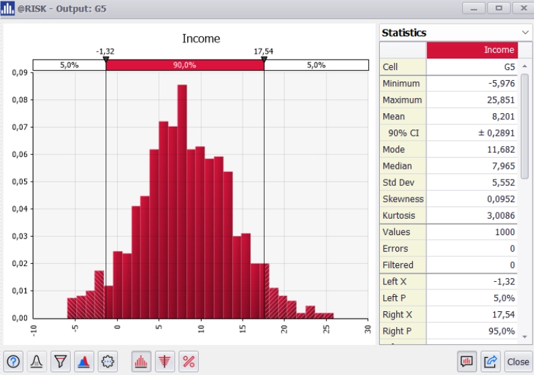
- Probability Distribution of Outcomes: Instead of a single answer, the simulation provides a histogram or probability density function showing the likelihood of various outcomes. For example, it might show that a software release has a 70% chance of being completed within budget, a 20% chance of exceeding it by 10%, and a 10% chance of exceeding it significantly.
- Average/Expected Value: The mean of the simulated outcomes provides a central tendency, an average expectation for the system’s performance.
- Confidence Intervals: These indicate the range within which the actual outcome is likely to fall with a certain level of confidence (e.g., 95% of project completions will fall between 8 and 12 months).
- Risk Assessment: Critical thresholds can be identified. For example, what is the probability that the system’s response time will exceed 500ms? What is the likelihood of a critical component failing within its warranty period?
- Sensitivity Analysis: By selectively varying the distributions of individual input variables and observing the change in the output distribution, analysts can determine which inputs have the greatest impact on the system’s behavior. This helps in prioritizing efforts to reduce uncertainty in the most influential areas.
Key Applications in Technology

Monte Carlo analysis is not just a theoretical concept; it’s a practical workhorse across numerous technology domains, enabling better decision-making and more robust system designs.
Software Development and Performance Testing
In software engineering, Monte Carlo methods are invaluable for estimating project timelines, budget overruns, and resource allocation under uncertainty. For example, tasks in a project plan rarely take a precise amount of time; they often have optimistic, most likely, and pessimistic estimates. A Monte Carlo simulation can run through thousands of possible project paths, considering these probabilistic task durations, to predict the overall project completion date with a probability distribution, identifying the likelihood of meeting deadlines or exceeding budgets.
Beyond project management, it’s used in performance testing and capacity planning. By simulating varying user loads, transaction rates, and network latencies, developers can predict how a new application or server infrastructure will perform under different real-world conditions, helping to identify bottlenecks and optimize resource provisioning before deployment.
Artificial Intelligence and Machine Learning
Monte Carlo techniques are foundational in many areas of AI and machine learning. In reinforcement learning, Monte Carlo methods are used to estimate the value functions of states or actions by simulating episodes of interaction with an environment. This helps an AI agent learn optimal policies in complex, uncertain environments like game playing (e.g., AlphaGo’s success with Monte Carlo Tree Search) or robotic control.
Furthermore, Monte Carlo methods are used in Bayesian inference, enabling approximate sampling from complex posterior distributions that are otherwise intractable. This is critical for training probabilistic models, estimating model parameters, and quantifying uncertainty in predictions made by AI systems. They are also employed in tasks like generative modeling, where new data points are sampled based on learned distributions.
Engineering and Design Optimization
In various engineering disciplines, Monte Carlo simulations are indispensable for reliability analysis, risk assessment, and design optimization. For example, when designing a complex electronic circuit, there are manufacturing tolerances for each component (resistors, capacitors, etc.). A Monte Carlo analysis can simulate thousands of circuits with randomly varying component values within their tolerance ranges to predict the overall performance, yield, and failure rates of the circuit. This helps engineers design more robust systems that function reliably despite inherent variability in their constituent parts. In aerospace, it can simulate the trajectory of spacecraft, accounting for atmospheric variations, thruster inaccuracies, and gravitational perturbations, to calculate the probability of successful mission outcomes.
Scientific Computing and Research
For scientific researchers, Monte Carlo methods provide a powerful tool for modeling complex physical, chemical, or biological systems that are too intricate for analytical solutions. For instance, in materials science, it can simulate the behavior of atoms and molecules to predict material properties. In computational biology, it’s used to model protein folding, DNA interactions, and population dynamics. Nuclear physics extensively uses Monte Carlo methods to simulate particle transport and interactions within nuclear reactors or radiation shielding. The ability to model inherently stochastic processes, such as particle decay or molecular motion, makes Monte Carlo analysis an essential instrument in modern scientific discovery.
Advantages and Considerations
While undeniably powerful, Monte Carlo analysis, like any advanced computational technique, comes with its own set of advantages and challenges that tech professionals must consider.
Handling Complexity and Non-Linearity
One of the greatest strengths of Monte Carlo analysis is its ability to handle extremely complex models with numerous interacting variables, non-linear relationships, and intricate dependencies. Unlike many analytical methods that require simplifying assumptions about linearity or independence, Monte Carlo simulations directly incorporate these complexities by simulating them. This makes it particularly suited for real-world technological systems that rarely conform to neat, simple equations. It can also effectively propagate uncertainty through multiple stages of a process, providing a holistic view of cumulative risk or variability.
Computational Demands and Efficiency
The primary drawback of Monte Carlo analysis is its computational cost. To achieve accurate and statistically significant results, a large number of simulations are required, often thousands to millions of runs. Each run, in turn, can involve complex calculations. This demands significant processing power and time, especially for highly detailed or large-scale models. While modern computing resources have made this more feasible, efficient algorithm design, parallel processing, and variance reduction techniques are often employed to speed up convergence and make simulations more practical. Cloud computing and distributed systems are increasingly leveraged to overcome these computational hurdles, allowing researchers and engineers to run massive simulations without prohibitive local hardware costs.
The Importance of Good Input Data
The adage “garbage in, garbage out” is particularly true for Monte Carlo analysis. The quality and accuracy of the simulation’s output are directly dependent on the quality of the input probability distributions. If the chosen distributions for uncertain variables do not accurately reflect reality, or if critical uncertain variables are overlooked, the simulation results will be misleading. Therefore, significant effort must be invested in data collection, statistical analysis, and expert judgment to establish reliable input distributions. This often involves historical data analysis, fitting distributions to observed frequencies, or eliciting expert opinions when historical data is scarce. Without a rigorous approach to input data, even the most sophisticated Monte Carlo model will fail to provide meaningful insights.
In conclusion, Monte Carlo analysis stands as a cornerstone in the arsenal of computational tools for anyone working with systems characterized by inherent uncertainty. Its ability to simulate countless scenarios and provide a probabilistic range of outcomes empowers better decision-making, more robust designs, and a deeper understanding of complex technological challenges, from software development to the frontiers of AI and scientific research.
aViewFromTheCave is a participant in the Amazon Services LLC Associates Program, an affiliate advertising program designed to provide a means for sites to earn advertising fees by advertising and linking to Amazon.com. Amazon, the Amazon logo, AmazonSupply, and the AmazonSupply logo are trademarks of Amazon.com, Inc. or its affiliates. As an Amazon Associate we earn affiliate commissions from qualifying purchases.