How to Graph x = 3: A Fundamental Guide to Vertical Lines

In the expansive world of mathematics and data visualization, graphing serves as a universal language, transforming abstract equations into tangible visual representations. For beginners and seasoned professionals alike, understanding how to graph even the simplest equations is a foundational skill that underpins more complex analytical tasks. One such seemingly straightforward equation is x = 3. While simple, its implications and proper representation are crucial, especially when moving towards digital tools and software-assisted plotting. This guide will delve into the technicalities of graphing x = 3, exploring both manual methods and the power of modern graphing technology, firmly positioning this tutorial within the realm of tech-driven education.

Table of Contents

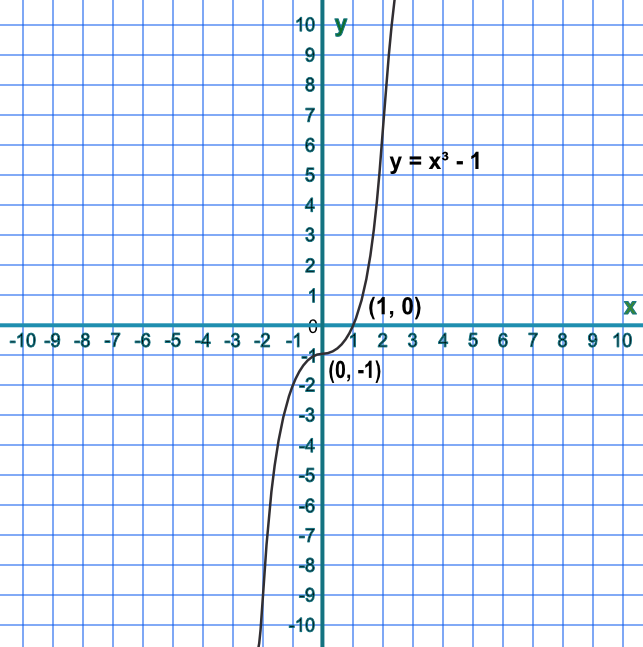
Understanding the Cartesian Coordinate System: The Canvas for Graphing

Before we can effectively graph any equation, including x = 3, it’s imperative to have a solid grasp of the canvas upon which we’ll be drawing: the Cartesian coordinate system. Developed by René Descartes, this system provides a structured framework for locating points in a two-dimensional plane, forming the bedrock for all graphical analysis in algebra and beyond.

The Basics of Axes and Origin

The Cartesian plane is defined by two perpendicular number lines:

The Horizontal Axis (x-axis): This line runs left to right and represents values along the independent variable, often denoted as x. Positive values extend to the right from the center, and negative values extend to the left.
The Vertical Axis (y-axis): This line runs up and down and represents values along the dependent variable, often denoted as y. Positive values extend upwards from the center, and negative values extend downwards.

The point where these two axes intersect is called the origin, denoted by the coordinates (0, 0). This point serves as the reference for all other points on the plane. Each axis is typically marked with evenly spaced increments (e.g., 1, 2, 3, … or -1, -2, -3, …), allowing for precise measurement and plotting. Understanding this fundamental setup is the first critical step in any graphing endeavor, whether performed manually with paper and pencil or digitally using sophisticated software.

How Points are Represented: The (x, y) Pair

Every unique location on the Cartesian plane is identified by an ordered pair of numbers, conventionally written as (x, y). The first number in the pair, x, specifies the horizontal position relative to the origin, while the second number, y, specifies the vertical position. For instance:

A point (2, 5) would be located by moving 2 units to the right from the origin along the x-axis, and then 5 units up parallel to the y-axis.
A point (-3, 1) would involve moving 3 units to the left along the x-axis, and then 1 unit up.
A point (0, 4) is on the y-axis, 4 units up from the origin.
A point (6, 0) is on the x-axis, 6 units to the right from the origin.

This (x, y) notation is universal across all graphing contexts, from elementary school mathematics to advanced engineering simulations. When we graph an equation, we are essentially finding all the (x, y) pairs that satisfy that equation and then connecting them to form a visual line or curve. This structured approach to spatial representation is a cornerstone of analytical geometry and a prerequisite for leveraging any graphing technology effectively.

Deciphering the Equation `x = 3`: The Nature of a Vertical Line

With the Cartesian system understood, we can now turn our attention to the specific equation x = 3. While many equations involve both x and y variables (like y = 2x + 1 or x^2 + y^2 = 9), x = 3 is unique because it only specifies a value for x. This singular constraint dictates a very particular and important type of line.

What `x = k` Means

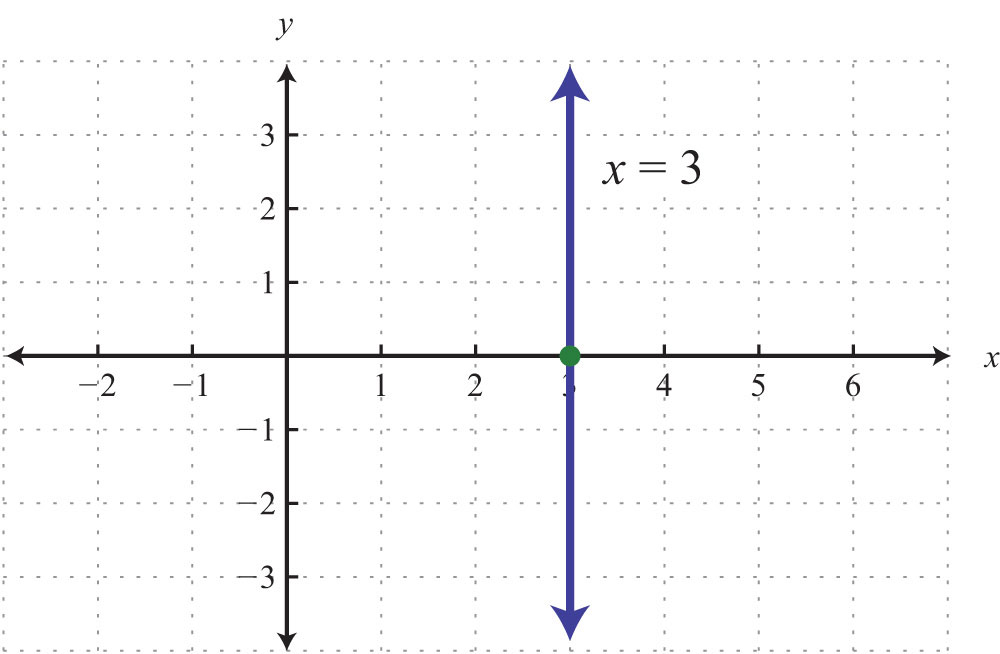
In general, an equation of the form x = k, where k is any constant number, represents a vertical line. This is because the equation states that every single point on the line must have an x-coordinate equal to k, regardless of its y-coordinate. In our specific case, x = 3, this means that every point that satisfies this equation must have an x-value of 3.

Consider a few points that would satisfy this condition:

If y = 0, then x must be 3. So, (3, 0) is a point on the line.
If y = 2, then x must be 3. So, (3, 2) is a point on the line.
If y = -1, then x must be 3. So, (3, -1) is a point on the line.
If y = 100, then x must be 3. So, (3, 100) is a point on the line.

No matter what value y takes, x will always be fixed at 3. This constant x-value, while y varies freely, is the defining characteristic of a vertical line.

The Invariance of the X-Coordinate

The concept of invariance is key here. For the equation x = 3, the x-coordinate is invariant. It does not change. This is a powerful concept in mathematics and computer science, especially when defining constraints or boundaries. In graphical terms, it means the line will always be parallel to the y-axis because its horizontal position never deviates from x = 3.

This understanding is critical not just for manual plotting but also for interpreting how graphing software handles such equations. When you input x = 3 into a digital graphing tool, the underlying algorithms recognize this invariant property and render a perfectly vertical line, demonstrating its mastery of these fundamental mathematical concepts. This simplification of complex patterns into elegant visual representations is precisely where technology shines.

Step-by-Step Manual Graphing for Foundational Understanding

Before jumping into digital tools, grasping the manual graphing process for x = 3 solidifies foundational understanding. This traditional method helps build intuition and provides a clear mental model that aids in interpreting digital outputs.

Setting Up Your Graph Paper

Draw Your Axes: Use a ruler to draw a horizontal line (x-axis) and a vertical line (y-axis) that intersect, forming your origin (0,0). Ensure they are perpendicular.
Label Axes: Clearly label the horizontal axis as x and the vertical axis as y.
Mark Scales: Add evenly spaced tick marks along both axes. Choose an appropriate scale (e.g., each square represents 1 unit). Label key numerical values (e.g., 1, 2, 3, -1, -2, -3, etc.) to ensure clarity.

Plotting Key Points

Since x = 3 means x is always 3, we can pick any y values and the x will remain constant.

Choose y-values: Select a few distinct y-values. Good choices are 0, a positive value, and a negative value to show the line extends indefinitely.
- Let y = 0: The point is (3, 0).
- Let y = 2: The point is (3, 2).
- Let y = -3: The point is (3, -3).
Plot the Points: Locate each of these ordered pairs on your Cartesian plane and mark them with a clear dot or small cross.
- For (3, 0): Move 3 units right from the origin on the x-axis, stay on the axis.
- For (3, 2): Move 3 units right, then 2 units up.
- For (3, -3): Move 3 units right, then 3 units down.

Drawing the Line and Labeling

Connect the Points: Once you have plotted at least two points (three is often better for accuracy checks), use your ruler to draw a straight line that passes through all of them. Extend the line beyond your plotted points to indicate that it continues infinitely in both directions.
Add Arrows: Place arrowheads at both ends of the line to visually signify its infinite extent.
Label the Line: Write the equation x = 3 near the line to clearly identify it.

This manual process, while seemingly simple, reinforces the spatial relationship between the equation and its geometric representation, a crucial precursor to engaging with more advanced tech tools.

Leveraging Digital Tools for Precision and Efficiency

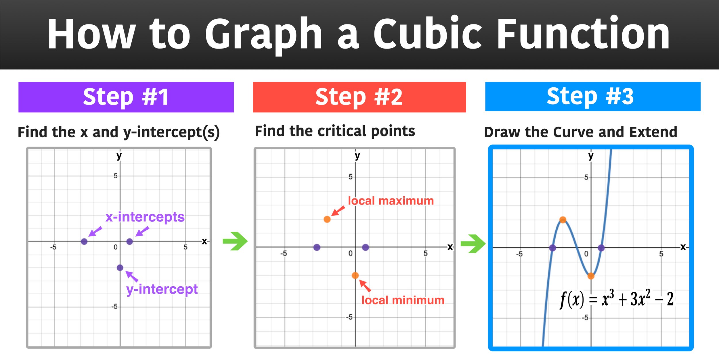
While manual graphing is essential for conceptual understanding, digital graphing tools offer unparalleled precision, speed, and advanced functionalities. These tools are indispensable in academic settings, engineering, data science, and any field requiring accurate visualization of mathematical relationships.

Introduction to Online Graphing Calculators (Desmos, GeoGebra)

Modern web-based graphing calculators have revolutionized how we interact with mathematical concepts.

Desmos Graphing Calculator: This intuitive, free online tool allows users to input equations directly. Simply type x = 3 into the input bar, and Desmos will instantly render the perfectly vertical line. It also allows for interactive exploration, letting you see how changing the constant (e.g., to x = 5) shifts the line. Its user-friendly interface makes it ideal for students and educators.
GeoGebra: Another powerful and free dynamic mathematics software, GeoGebra combines geometry, algebra, spreadsheets, graphing, statistics, and calculus in one easy-to-use package. Entering x = 3 in GeoGebra’s input field yields the same vertical line, with additional options for customizing its appearance, adding labels, and even integrating it into more complex geometric constructions.

These platforms not only graph x = 3 but can also handle functions, inequalities, parametric equations, and even 3D graphing, offering a rich environment for mathematical exploration.

Using Scientific and Graphing Calculators (TI-84, Casio)

For those in exam settings or without immediate internet access, dedicated graphing calculators remain vital.

TI-84 Plus (and similar TI models): While primarily designed for y = f(x) functions, the TI-84 can graph vertical lines using a parametric mode or by drawing a line segment. To graph x = 3 specifically, one often needs to use the “Draw” menu (e.g., 2nd -> PRGM (DRAW) -> 4:Vertical) and then input 3. This draws a vertical line at x = 3 across the entire screen. Some advanced models may allow direct x= input in certain modes.
Casio FX-CG50 (and similar Casio models): Casio’s color graphing calculators are also powerful. In the “Graph” menu, some models allow x= inputs directly, or you might navigate to a “Conics” or “Special Functions” menu to define vertical lines. The exact steps can vary by model, but the capability is generally present.

Mastering these physical graphing calculators is a key tech skill for students in higher mathematics and science courses.

Programming Approaches (Python with Matplotlib)

For those venturing into data science, engineering, or research, programmatic graphing offers the ultimate flexibility and automation.

Python with Matplotlib: Matplotlib is a comprehensive library for creating static, animated, and interactive visualizations in Python. To graph x = 3:

import matplotlib.pyplot as plt
import numpy as np

# Define the x-value for the vertical line
x_val = 3

# Define a range for y values (to make sure the line covers the plot area)
y_vals = np.linspace(-5, 5, 100) # From -5 to 5, 100 points

# Create a figure and an axes object
fig, ax = plt.subplots()

# Plot the vertical line
ax.plot([x_val, x_val], [y_vals.min(), y_vals.max()], color='blue', linestyle='--')

# Add a point on the x-axis for reference
ax.plot(x_val, 0, 'ro', markersize=5) # Red circle at (3,0)

# Set labels and title
ax.set_xlabel("X-axis")
ax.set_ylabel("Y-axis")
ax.set_title(f"Graph of x = {x_val}")

# Set grid
ax.grid(True)

# Set x and y limits for better visualization
ax.set_xlim(-5, 5)
ax.set_ylim(-5, 5)

# Add an annotation for the line
ax.text(x_val + 0.1, y_vals.max() * 0.8, f'x = {x_val}', rotation=90, va='center', color='blue')

# Show the plot
plt.axvline(x=x_val, color='red', linestyle='-', label=f'x = {x_val}') # A simpler way using axvline
plt.legend()
plt.show()

This code snippet demonstrates not only how to draw the line but also how to add labels, titles, grids, and customize its appearance, showcasing the power of programmatic control over visualizations.

The Significance and Applications of Vertical Lines

Beyond merely being a mathematical curiosity, vertical lines like x = 3 hold significant importance across various disciplines, serving as fundamental building blocks and representations of critical concepts.

Foundational Concepts in Algebra and Geometry

In algebra, understanding x = k and y = k (horizontal lines) is crucial for grasping the broader classification of linear equations. They represent special cases where one variable is constant, simplifying analysis. In geometry, vertical lines are parallel to the y-axis, define boundaries, and are integral to understanding transformations, symmetry, and geometric proofs. They are also essential when discussing concepts like domain and range of functions, where vertical lines can indicate restrictions (e.g., vertical asymptotes).

Real-World Scenarios (Constraints, Boundaries, Thresholds)

In practical applications, x = 3 (or any x = k) often represents a hard boundary, a fixed constraint, or a threshold.

Engineering: Imagine a structural beam fixed at a certain x-coordinate, or a design specification stating “component cannot extend beyond x = 3 meters.”
Computer Graphics: In game development or UI/UX design, x = 3 might define the edge of a game world, a UI element’s fixed position, or a viewport boundary. Pixels, by nature, are plotted on a discrete grid, mirroring the Cartesian plane.
Data Analysis: In statistical plots, a vertical line might represent a mean, a median, a control limit, or a decision boundary in classification algorithms (e.g., “if x > 3, then classify as A; otherwise, classify as B”).
Logistics: A factory might have a processing stage that occurs precisely at a designated physical location x = 3 on its assembly line.

These examples underscore that graphing x = 3 isn’t just an academic exercise but a practical skill for visualizing constraints and understanding spatial relationships in technology and real-world systems.

Common Mistakes and How to Avoid Them

Even with simple equations, common pitfalls can occur:

Confusing x = 3 with y = 3: A frequent mistake is to graph x = 3 as a horizontal line. Remember, x values are horizontal, so x = 3 means the line passes through the x-axis at 3 and goes vertically. Conversely, y = 3 is a horizontal line.
Not Extending the Line: A common error in manual graphing is drawing only a segment. Lines extend infinitely, so always add arrows to indicate this. Digital tools handle this automatically, drawing lines to the edges of the defined plot.
Incorrect Scaling: If axes are not scaled consistently or clearly labeled, the graph can be misleading. Digital tools typically auto-scale or allow easy adjustment of viewports, reducing this manual error.
Misinterpreting “No y variable”: Some might incorrectly think x = 3 is just a point. It’s an equation that describes an infinite set of points where x is always 3, making it a line.

By understanding these common errors and the foundational principles, one can accurately and confidently graph x = 3 using both traditional methods and the array of powerful digital tools available today, solidifying a crucial skill in the tech-driven landscape of data visualization and mathematical analysis.

aViewFromTheCave is a participant in the Amazon Services LLC Associates Program, an affiliate advertising program designed to provide a means for sites to earn advertising fees by advertising and linking to Amazon.com. Amazon, the Amazon logo, AmazonSupply, and the AmazonSupply logo are trademarks of Amazon.com, Inc. or its affiliates. As an Amazon Associate we earn affiliate commissions from qualifying purchases.