How to Graph in a Graphing Calculator: A Comprehensive Tutorial

The graphing calculator stands as an indispensable tool in the arsenals of students, educators, engineers, and scientists alike. Far from being a mere calculator, these sophisticated devices transform abstract mathematical equations into tangible visual representations, offering profound insights into functions, data, and complex relationships. Mastering your graphing calculator isn’t just about pressing buttons; it’s about unlocking a powerful visual language that can clarify concepts, solve intricate problems, and deepen understanding across various STEM disciplines.

In an age where technology continually reshapes our learning and problem-solving approaches, the graphing calculator remains a cornerstone for its ability to bridge the gap between theoretical mathematics and practical application. Whether you’re navigating high school algebra, college calculus, or professional engineering tasks, the capacity to quickly and accurately visualize functions is invaluable. This comprehensive tutorial aims to demystify the process, guiding you from the basic setup to advanced graphing techniques, ensuring you can harness the full potential of your device. We’ll explore the essential functions, common pitfalls, and best practices, empowering you to confidently interpret and manipulate graphical data.

Understanding Your Graphing Calculator’s Anatomy

Before diving into the mechanics of graphing, it’s crucial to familiarize yourself with the layout and core functionalities of your graphing calculator. While specific models (like TI-83, TI-84 Plus, Casio fx-9750GII, etc.) may have slightly different button placements or menu structures, the fundamental principles remain consistent.

Keypad Layout and Essential Buttons

Your calculator’s keypad is organized logically, with numerical keys, operational keys (+, -, *, /), and a host of specialized function keys. For graphing, several buttons are paramount:

Y=: This button opens the “Y-editor” (or function editor) where you input the equations you wish to graph. You’ll typically see Y1=, Y2=, etc., allowing you to graph multiple functions simultaneously.
WINDOW: This key is critical for defining the range and scale of your graph. It allows you to set the minimum and maximum values for both the x and y axes (Xmin, Xmax, Ymin, Ymax), as well as the tick mark intervals (Xscl, Yscl). Understanding the window settings is often the key to seeing your graph correctly.
ZOOM: The ZOOM menu provides various options to adjust the viewing window quickly. Common options include ZoomStandard (a default -10 to 10 range for both axes), ZoomFit (adjusts Y-values to show the entire function within the current X-range), ZoomIn, ZoomOut, and ZoomSquare.
GRAPH: Once an equation is entered and the window is set, pressing this button displays the graph on the screen.
TRACE: After a graph is displayed, the TRACE button allows you to move a cursor along the curve, showing the corresponding x and y coordinates. This is incredibly useful for exploring function values.
2nd (or Shift): This key accesses the secondary functions printed above many of the primary buttons. For instance, 2nd + TRACE often opens the CALC (calculate) menu, which is vital for finding intersections, zeros, minimums, and maximums.

Screen Display and Interpretation

The calculator’s screen is where all the magic happens. It typically features a pixelated grid where functions are plotted. Learning to interpret this display involves understanding:

Axes: The horizontal line represents the x-axis, and the vertical line represents the y-axis. Their intersection is the origin (0,0).
Grids and Tick Marks: Depending on your WINDOW settings, you’ll see tick marks along the axes, and sometimes a full grid, helping you estimate coordinates.
Cursor: When using TRACE or other analysis tools, a blinking cursor will appear on the graph, indicating the specific point being examined.

Menu Navigation and Mode Settings

Modern graphing calculators are replete with menus (e.g., MODE, FORMAT, CALC, STAT, PRGM). The MODE button is particularly important for graphing, as it allows you to switch between different types of graphing environments:

Function Mode (Func): This is the default and most commonly used mode for graphing functions of the form Y = f(X).
Parametric Mode (Par): Used for graphing equations defined by a parameter (e.g., X = f(T), Y = g(T)).
Polar Mode (Pol): For graphing polar equations (e.g., r = f(θ)).
Sequence Mode (Seq): For graphing sequences and series.

Always ensure your calculator is in the correct mode for the type of equation you intend to graph. Incorrect mode settings are a frequent source of frustration for new users.

The Fundamentals of Graphing Functions

With a basic understanding of your calculator’s anatomy, you can now proceed to the core process of graphing a function. This involves a straightforward sequence of steps that will become second nature with practice.

Entering Equations (Y= Editor)

Press Y=: This opens the function editor.
Select a Function Slot: Choose an available Y#= slot (e.g., Y1=). If a slot is already occupied, you can clear the existing equation by moving the cursor to that line and pressing CLEAR.
Input Your Equation: Type your function using the variable X (typically accessed via a dedicated X,T,θ,n button). For example, to graph y = 2x + 3, you would type 2X + 3. Be mindful of parentheses for complex expressions (e.g., (X+1)/(X-2)). Use the negative sign (-) for subtraction and the unary minus key (often a small grey button) for negative numbers.

Setting the Viewing Window (WINDOW Settings)

This is perhaps the most crucial step after entering the equation. If your window is not set appropriately, you might not see your graph at all, or only a small, uninformative part of it.

Press WINDOW: This brings up the window settings menu.
Adjust Parameters:
- Xmin: The smallest x-value displayed on the graph.
- Xmax: The largest x-value displayed on the graph.
- Xscl: The interval between tick marks on the x-axis.
- Ymin: The smallest y-value displayed on the graph.
- Ymax: The largest y-value displayed on the graph.
- Yscl: The interval between tick marks on the y-axis.
Consider Your Function: For y = 2x + 3, a standard window (like Xmin=-10, Xmax=10, Ymin=-10, Ymax=10) is usually sufficient. However, for functions like y = x^2 + 100, you’d need a much larger Ymax to see the vertex. For trigonometric functions, you might set Xmin=0, Xmax=2π (using 2*PI from the 2nd + ^ menu) and Xscl=PI/2.

Displaying the Graph (GRAPH Button)

Once your equation is entered and your window is set, simply press the GRAPH button. Your calculator will plot the function on the screen according to your specified window parameters. If you don’t see anything, revisit your WINDOW settings or try one of the ZOOM options.

Adjusting the Zoom (ZOOM Menu)

The ZOOM menu offers quick ways to adjust your view:

Press ZOOM:
Select an Option:
- ZoomStandard (option 6): Sets the window to Xmin=-10, Xmax=10, Ymin=-10, Ymax=10. A great starting point.
- ZoomFit (option 0 or 10): Calculates appropriate Ymin and Ymax values to ensure the entire range of the function is visible within the current Xmin/Xmax settings. Highly useful when you know the x-range but not the y-range.
- ZoomIn/ZoomOut: Allows you to magnify or de-magnify a specific area. After selecting ZoomIn/ZoomOut, use the arrow keys to move the cursor to the desired center of the zoom, then press ENTER.
- ZoomSquare: Adjusts the aspect ratio so that units on the x-axis and y-axis are scaled equally, preventing distortion of shapes (e.g., circles appearing as ellipses).

Advanced Graphing Techniques and Analysis

Graphing calculators excel not just at displaying functions but also at analyzing them. These advanced features are where the true power of visualization comes into play.

Graphing Multiple Functions

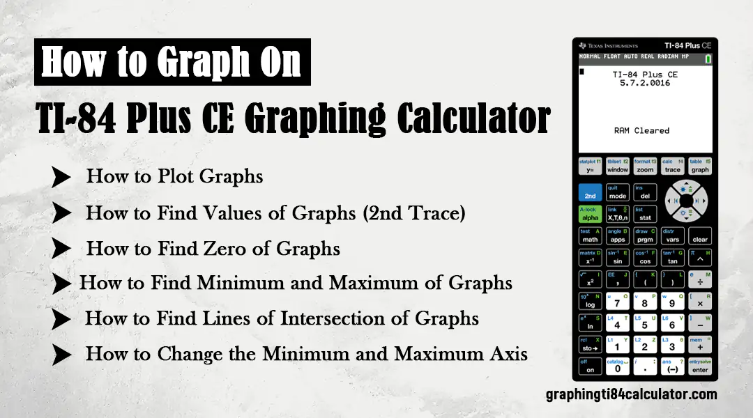
To graph more than one function at a time, simply enter additional equations into the Y= editor (e.g., Y1=, Y2=, Y3=). The calculator will plot them all, usually in different colors or line styles, allowing for direct comparison and analysis of their relationships.

Tracing and Finding Intersections

The TRACE function (press TRACE button) allows you to move a cursor along a displayed graph, showing the x and y coordinates at each point. If multiple graphs are present, use the up/down arrow keys to jump between them.

For precise analysis, the CALC menu (2nd + TRACE) is invaluable:

value (option 1): Enter an x-value to find the corresponding y-value on the selected graph.
zero (option 2): Finds the x-intercepts (roots) of a function. You’ll need to specify a “Left Bound” and “Right Bound” (points on either side of the zero) and a “Guess”.
minimum (option 3) / maximum (option 4): Finds the local minimum or maximum points of a function within a specified range (Left Bound, Right Bound, Guess).
intersect (option 5): Finds the point(s) where two or more graphs cross. Select the “First Curve,” “Second Curve,” and provide a “Guess” near the intersection. This is incredibly useful for solving systems of equations graphically.

Exploring Inequalities and Shading

While some calculators have direct inequality graphing functions, a common workaround involves shading:

Enter the Boundary Function: Input the equation of the line/curve (e.g., Y1 = -X + 5).
Adjust Line Style/Shading: Go to the Y= editor, move the cursor to the far left of the Y1= line, and press ENTER repeatedly to cycle through different line styles. You’ll find options for shading above (for y > f(x) or y >= f(x)) or below (for y < f(x) or y <= f(x)).
Graph: Press GRAPH to see the shaded region. For systems of inequalities, you might need to use a combination of shading techniques or explore more advanced app functionalities if available on your calculator.

Parameterizing and Polar Coordinates

Switching modes in the MODE menu (as discussed earlier) allows you to graph in different coordinate systems.

Parametric: In Par mode, the Y= editor changes to X1T=, Y1T=, etc. You’ll input expressions for x and y in terms of T (the variable button changes from X to T). You’ll also need to set Tmin, Tmax, and Tstep in the WINDOW settings.
Polar: In Pol mode, the Y= editor changes to r1=, r2=, etc. You’ll input expressions for r in terms of θ (the variable button changes to θ). WINDOW settings will include θmin, θmax, and θstep.

These modes are essential for visualizing complex curves that cannot be expressed easily as y = f(x).

Common Pitfalls and Troubleshooting Tips

Even experienced users encounter issues. Knowing how to diagnose and resolve common problems can save significant time and frustration.

“ERR: WINDOW RANGE” and Other Error Messages

ERR: WINDOW RANGE: This typically means your Xmin is greater than Xmax, or Ymin is greater than Ymax. Go to WINDOW and correct these values.
ERR: DOMAIN: You’re trying to calculate a value or graph a function outside its defined domain (e.g., sqrt(-1) or log(0)). Adjust your WINDOW or function input.
ERR: SYNTAX: An error in how you’ve typed the equation. Check for unmatched parentheses, missing operators, or incorrect function syntax.
ERR: OVERFLOW / ERR: DIVIDE BY 0: The calculation results in a number too large for the calculator, or you’re attempting to divide by zero.

Graph Not Showing or Invisible

This is usually a WINDOW issue:

Function outside the window: The graph exists but is outside the currently defined Xmin, Xmax, Ymin, Ymax. Try ZoomStandard or ZoomFit.
Graph is a straight vertical line: Your Xmin and Xmax are too close, or Xscl is too large.
Mode setting is incorrect: You’re trying to graph a polar equation in Function mode, for instance. Check MODE.
Function is deselected: In the Y= editor, ensure the equals sign (=) next to your function is highlighted. If it’s not, move the cursor to the equals sign and press ENTER to select/deselect it.

Resetting Your Calculator

Sometimes, the quickest fix for persistent issues or unexpected behavior is to reset your calculator to its default settings. This varies by model but often involves a 2nd + MEM (Memory) menu, then selecting Reset or Defaults. Be aware that this will erase all stored programs and variables.

Beyond Basic Graphing: Applications and Best Practices

Mastering basic graphing is just the beginning. Graphing calculators are powerful tools that can extend your mathematical understanding and problem-solving capabilities.

Data Plotting and Statistics

Many graphing calculators can plot statistical data (scatter plots, box plots, histograms) and perform regression analysis. This typically involves entering data into STAT lists and then selecting a STAT PLOT option. Visualizing data alongside regression lines can greatly aid in understanding trends and relationships.

Solving Equations Graphically

As demonstrated with the intersect feature, you can solve equations by graphing. To solve f(x) = g(x), graph Y1 = f(x) and Y2 = g(x), then find their intersection points. To solve f(x) = 0, graph Y1 = f(x) and find its zeros (x-intercepts). This graphical approach provides a powerful complement to algebraic methods, offering immediate visual confirmation of solutions.

The Role of Graphing Calculators in STEM Education

Graphing calculators serve as dynamic learning environments. They allow students to:

Explore “What If” Scenarios: Instantly see how changing parameters in an equation affects its graph.
Visualize Abstract Concepts: Bring functions, derivatives, integrals, and statistical distributions to life.
Develop Intuition: Build a deeper understanding of mathematical relationships through visual exploration.
Solve Real-World Problems: Apply mathematical models to practical situations and analyze their graphical outputs.

Best Practices:

Practice Regularly: The more you use your calculator, the more intuitive its functions will become.
Read Your Manual: Your calculator’s user manual is an invaluable resource for specific features and troubleshooting.
Experiment: Don’t be afraid to try different settings and functions. Learning by doing is highly effective.
Backup Your Work: If your calculator supports it, back up programs and important data to a computer, especially before a reset.

In conclusion, the graphing calculator is far more than a simple computation device; it’s a dynamic visualizer that empowers users to explore, understand, and solve complex mathematical problems. By thoroughly understanding its anatomy, mastering fundamental graphing techniques, and leveraging advanced analytical tools, you can transform your approach to mathematics and science. Embrace the power of visualization, and let your graphing calculator be your guide to a deeper, more intuitive grasp of the quantitative world.

aViewFromTheCave is a participant in the Amazon Services LLC Associates Program, an affiliate advertising program designed to provide a means for sites to earn advertising fees by advertising and linking to Amazon.com. Amazon, the Amazon logo, AmazonSupply, and the AmazonSupply logo are trademarks of Amazon.com, Inc. or its affiliates. As an Amazon Associate we earn affiliate commissions from qualifying purchases.