How to Find the Function of a Graph

Understanding the underlying mathematical function that describes a given graph is a cornerstone skill in numerous technological and scientific disciplines. Whether you’re a data scientist analyzing trends, an engineer modeling physical systems, a software developer implementing algorithms, or a researcher interpreting experimental results, the ability to translate visual data into an algebraic expression is invaluable. This process, often referred to as curve fitting or regression analysis, bridges the gap between raw data points and a predictive, interpretable model.

In the era of big data and artificial intelligence, this capability extends beyond manual plotting to sophisticated computational methods. This article delves into a comprehensive guide on how to find the function of a graph, moving from fundamental visual inspection to leveraging advanced software tools and machine learning techniques, all strictly within the domain of technology.

Table of Contents

Understanding the Fundamentals: Visual Inspection and Basic Forms

Before diving into complex algorithms, the first step in identifying a graph’s function is often a keen visual inspection. Our eyes are excellent pattern recognition tools, and familiarizing oneself with the visual signatures of common mathematical functions is crucial.

Recognizing Common Graph Shapes

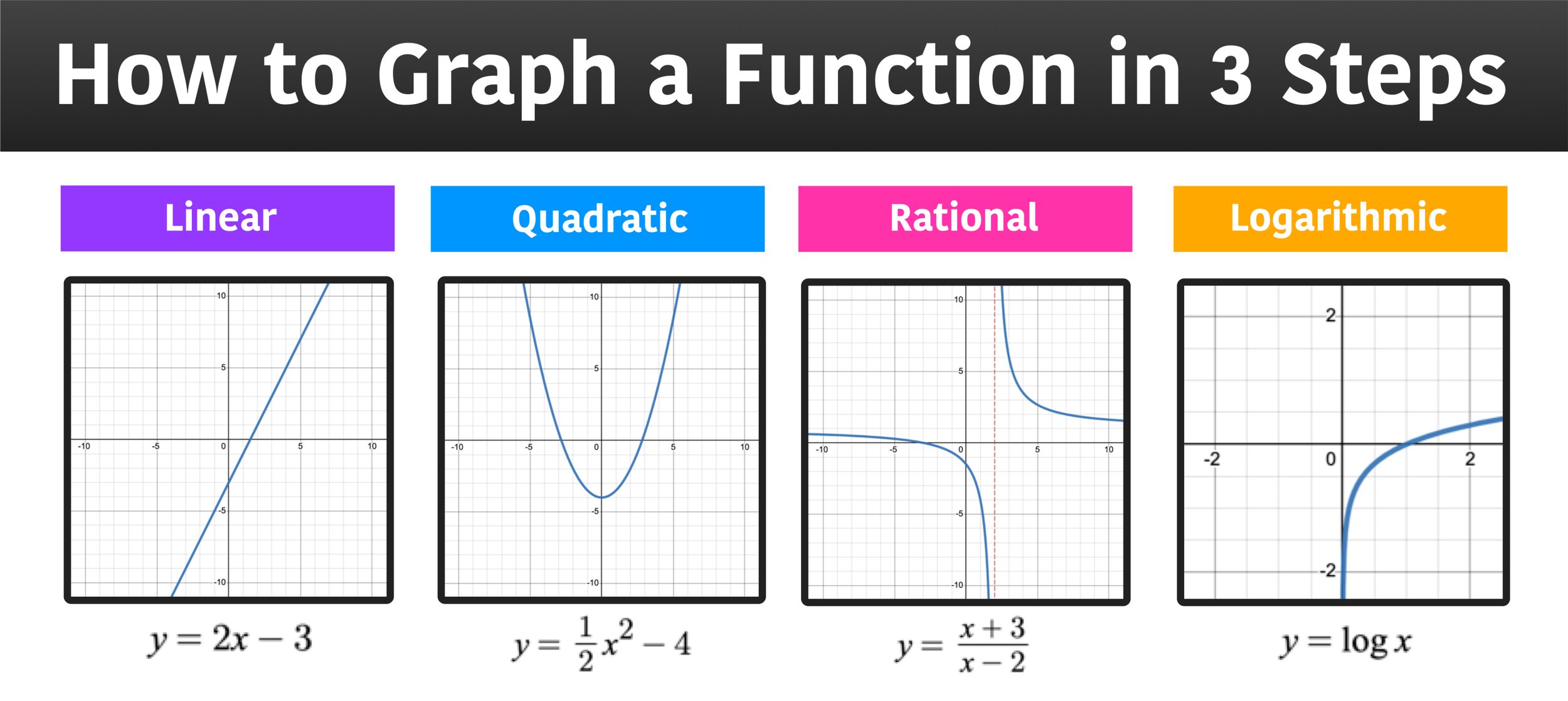
Different functions produce distinct graphical patterns. Being able to quickly identify these archetypes provides a strong starting point for formal analysis:

Linear Functions ($y = mx + b$): Characterized by a perfectly straight line. The ‘m’ represents the slope (rate of change), and ‘b’ is the y-intercept (where the line crosses the y-axis).
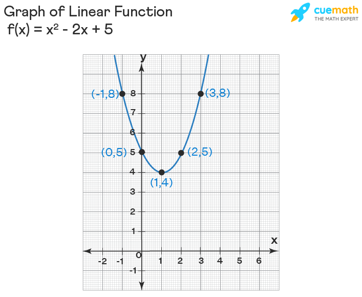
Quadratic Functions ($y = ax^2 + bx + c$): These form parabolas, which are U-shaped curves opening either upwards (if ‘a’ > 0) or downwards (if ‘a’ < 0).
Exponential Functions ($y = ab^x$): Exhibit rapid growth or decay. The curve typically gets steeper or flatter at an increasing rate, never touching the x-axis (asymptote).
Logarithmic Functions ($y = a log(x) + b$): The inverse of exponential functions. They typically grow slowly and then level off, never touching the y-axis.
Power Functions ($y = ax^n$): A broad category including many polynomial forms. For instance, $y = x^3$ forms an S-shape, while $y = x^2$ is a parabola.
Sinusoidal Functions ($y = A sin(Bx + C) + D$ or $y = A cos(Bx + C) + D$): Represent periodic, wave-like patterns, common in oscillations and cycles. Key features include amplitude, period, phase shift, and vertical shift.

Identifying Key Features

Beyond the overall shape, specific features on a graph provide critical clues for function determination:

Intercepts: Points where the graph crosses the x-axis (x-intercepts, where $y=0$) or y-axis (y-intercept, where $x=0$).
Slope/Rate of Change: How steeply the graph rises or falls. Constant for linear functions, changing for non-linear ones.
Vertex/Turning Points: The maximum or minimum points on curves like parabolas or other polynomials.
Asymptotes: Lines that the graph approaches but never quite touches, indicating limits or undefined regions.
Periodicity: For wave functions, the length of one complete cycle.

By carefully observing these characteristics, one can often make an educated guess about the family of functions the graph belongs to, significantly narrowing down the search for its precise equation.

Manual Methods: From Points to Equations

Once a likely function family is identified, basic algebraic methods can often be used to derive the exact equation, especially for simpler forms. These manual techniques form the foundation upon which automated software tools are built.

Linear Functions: The Two-Point Method

For a straight line, only two distinct points are needed to determine its equation.

Calculate the Slope (m): Choose any two points on the line, $(x1, y1)$ and $(x2, y2)$. The slope is $m = frac{y2 – y1}{x2 – x1}$.
Find the Y-intercept (b): Once ‘m’ is known, use one of the points and the slope in the slope-intercept form $y = mx + b$ to solve for ‘b’. For example, $b = y1 – mx1$.
Formulate the Equation: Combine ‘m’ and ‘b’ into the final equation $y = mx + b$.

Quadratic Functions: Using Three Points or Vertex Form

Quadratic functions require a bit more information.

Using Three Points: If you can identify three points $(x1, y1)$, $(x2, y2)$, and $(x3, y3)$ on the parabola, substitute each into the standard form $y = ax^2 + bx + c$. This creates a system of three linear equations with three unknowns (a, b, c) that can be solved simultaneously.
Using Vertex Form ($y = a(x-h)^2 + k$): If the vertex $(h, k)$ of the parabola is clearly identifiable, this form is often simpler. Plug in the vertex coordinates. Then, use one additional point $(x, y)$ on the parabola to solve for ‘a’.

Exponential and Logarithmic Functions: Transformation and Regression Principles

These functions are more complex to derive manually, but certain transformations can linearize them, allowing for linear regression techniques.

Exponential to Linear: For $y = ab^x$, taking the logarithm of both sides yields $log(y) = log(a) + x log(b)$. If you plot $log(y)$ against $x$, you should get a straight line. You can then find its slope ($log(b)$) and y-intercept ($log(a)$) and convert back to ‘a’ and ‘b’.
Power to Linear: For $y = ax^n$, taking the logarithm of both sides gives $log(y) = log(a) + n log(x)$. Plotting $log(y)$ against $log(x)$ will produce a straight line with slope ‘n’ and y-intercept $log(a)$.

These manual transformations highlight the core principles of regression, where data is fitted to a model by minimizing the distance between observed points and the model’s predictions.

Leveraging Technology: Software Tools and Libraries

Manual methods become cumbersome and prone to error with noisy data or complex functions. This is where technology shines, offering powerful tools for efficient and accurate function discovery.

Spreadsheet Software (Excel, Google Sheets)

For simple datasets, spreadsheets are an accessible entry point:

Plotting Data: Input your (x, y) data points and create a scatter plot.
Adding Trendlines: Most spreadsheet programs allow you to add a “trendline” to your chart. You can choose from linear, exponential, logarithmic, polynomial (up to a certain degree), and power trendlines.
Displaying Equation and R-squared: Crucially, you can usually check an option to “Display Equation on chart” and “Display R-squared value on chart.” The R-squared value indicates how well the trendline fits the data (closer to 1 is better).
While convenient, spreadsheet trendlines have limitations for highly complex or custom functions.

Programming Languages and Libraries (Python, R)

For serious data analysis, programming languages offer unparalleled flexibility and power.

Python:
- NumPy: The polyfit() function can find the coefficients of a polynomial of a specified degree that best fits the data.
- SciPy.optimize.curve_fit(): This is a highly versatile function that can fit data to any user-defined function. You provide your function (e.g., a custom exponential decay or a damped sine wave), initial parameter guesses, and your x and y data, and curve_fit will find the optimal parameters.
- Matplotlib and Seaborn: Essential for visualizing the data and the fitted function to assess the quality of the fit.
R:
- lm(): For linear models, including multiple linear regression.
- nls(): For non-linear least squares, allowing fitting of custom non-linear models.
- ggplot2: A powerful library for data visualization.

The advantages of programming lie in their ability to automate fitting across large datasets, handle complex custom functions, and integrate seamlessly into larger data processing pipelines.

Dedicated Math Software (MATLAB, Wolfram Alpha, GeoGebra)

Specialized software environments are designed for mathematical computation and visualization:

MATLAB: A powerful numerical computing environment. It offers extensive toolboxes for curve fitting (fit function), regression analysis, and symbolic mathematics. It’s particularly strong for engineering and scientific applications.
Wolfram Alpha: An online computational knowledge engine. You can directly input data points or describe a graph, and it can attempt to find the best-fit function, often displaying multiple possibilities and their goodness-of-fit metrics. It’s excellent for quick exploration and verification.
GeoGebra: An interactive geometry, algebra, statistics, and calculus application. It allows users to plot points, visualize functions, and perform curve fitting visually, which can be very intuitive for understanding the process.

AI-Powered Tools and Machine Learning Approaches

At the cutting edge, AI and machine learning offer increasingly sophisticated methods:

Regression Models: Beyond simple linear or polynomial regression, machine learning encompasses a wide array of regression algorithms (e.g., Ridge, Lasso, Support Vector Regression, Decision Trees, Random Forests, Gradient Boosting) that can model complex non-linear relationships without explicitly defining a function form. However, interpreting a single explicit mathematical function from these “black box” models can be challenging.
Symbolic Regression: This is a specific type of machine learning (often using genetic programming) that explicitly searches for the mathematical expression (the function) itself. Instead of just finding parameters for a pre-defined function, symbolic regression explores different combinations of mathematical operators, variables, and constants to evolve the best-fitting formula. This offers high interpretability, which is often a goal when “finding the function of a graph.”
Neural Networks: While primarily used for prediction, neural networks can approximate any continuous function (Universal Approximation Theorem). While they don’t typically output a simple equation, their ability to learn complex mappings means they are implicitly “finding the function” in a highly distributed and non-linear way. Techniques like feature importance or model interpretation tools can shed light on their learned relationships.

Best Practices and Advanced Considerations

Finding the “right” function is as much an art as it is a science. Several best practices enhance the accuracy and reliability of your results.

Data Preprocessing and Cleaning

Raw data is rarely perfect. Effective preprocessing is crucial:

Handling Noise and Outliers: Real-world data often contains random fluctuations (noise) or anomalous points (outliers). Techniques like smoothing (moving averages, Savitzky-Golay filters) can reduce noise, while outlier detection methods (e.g., Z-score, IQR method) help identify and potentially remove or mitigate their influence.
Missing Data: Decide how to handle missing data points (interpolation, imputation, or removal).
Normalization/Standardization: Scaling data can improve the performance of some fitting algorithms and machine learning models, especially those sensitive to feature scales.

Model Selection and Validation

Choosing the correct function and verifying its performance are critical steps:

Avoiding Overfitting: A common pitfall is choosing a function that is too complex for the data, fitting the noise rather than the underlying pattern. This leads to poor generalization on new data. The principle of Occam’s Razor suggests choosing the simplest model that adequately explains the data.
Using Metrics: Evaluate the goodness of fit using statistical metrics:
- R-squared (Coefficient of Determination): Explains the proportion of variance in the dependent variable predictable from the independent variable(s).
- RMSE (Root Mean Squared Error): Measures the average magnitude of the errors.
- MAE (Mean Absolute Error): Another measure of average error magnitude, less sensitive to outliers than RMSE.
Cross-Validation: Split your data into training and validation sets. Fit the function on the training set and evaluate its performance on the unseen validation set to get a more realistic assessment of its generalization ability.
Residual Analysis: Plot the residuals (the differences between actual and predicted y-values) against the independent variable. A good fit will show randomly scattered residuals, while patterns indicate that the model is missing important structure in the data.

Interpreting the Function and Its Limitations

Deriving an equation is only half the battle; understanding its implications and limitations is equally important:

Physical Meaning of Parameters: In many scientific and engineering contexts, the coefficients in your derived function have real-world meaning (e.g., growth rate, damping constant, initial value).
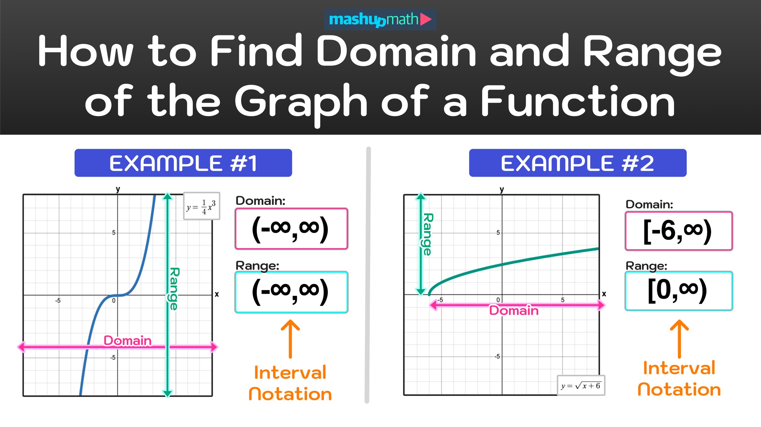
Extrapolation vs. Interpolation: Be cautious when extrapolating (predicting values outside the range of your observed data), as the model’s behavior might change significantly beyond the observed domain. Interpolation (predicting within the observed range) is generally safer.
Assumptions of the Model: Be aware of the underlying assumptions of the fitting method chosen (e.g., linearity, normally distributed errors). Violating these assumptions can invalidate your results.
Domain Knowledge is Crucial: Always integrate domain-specific knowledge into your analysis. Sometimes a visually perfect fit might be physically nonsensical, or a slightly worse statistical fit might be more interpretable and robust given the context.

Conclusion

The journey to find the function of a graph is a fundamental endeavor in the technological landscape, bridging visual data with analytical models. From the foundational skill of visual pattern recognition to the sophistication of manual algebraic derivations, and ultimately to the power of spreadsheet software, programming libraries, and advanced AI techniques like symbolic regression, the methods available are diverse and continually evolving.

Mastering these techniques empowers you to not just describe data but to understand its underlying mechanisms, make predictions, and build robust, data-driven applications. As technology continues to generate vast quantities of data, the ability to extract meaningful mathematical functions from graphs remains an indispensable skill for innovation and problem-solving across all tech-related fields. Embrace the tools and methodologies discussed, and continuously refine your analytical prowess to unlock the secrets hidden within every curve and line.

aViewFromTheCave is a participant in the Amazon Services LLC Associates Program, an affiliate advertising program designed to provide a means for sites to earn advertising fees by advertising and linking to Amazon.com. Amazon, the Amazon logo, AmazonSupply, and the AmazonSupply logo are trademarks of Amazon.com, Inc. or its affiliates. As an Amazon Associate we earn affiliate commissions from qualifying purchases.