What is the Matrix Equation?

In the vast and intricate landscape of modern technology, where algorithms power our every interaction and data shapes our understanding of the world, a seemingly abstract mathematical concept stands as a fundamental pillar: the matrix equation. Far from being a relic of academic textbooks, matrix equations are the silent workhorses behind everything from the stunning graphics in your favorite video game to the sophisticated intelligence of AI systems and the intricate analyses performed on massive datasets. Understanding “what is the matrix equation” is not just a mathematical curiosity; it’s a key to unlocking a deeper comprehension of how contemporary technology functions and innovates.

At its heart, a matrix equation represents a system of linear equations in a compact and elegant form. It provides a powerful framework for solving complex problems involving multiple variables and interdependencies, making it indispensable across virtually every domain within the tech sector. This article will demystify the matrix equation, breaking down its components, exploring its significance, and illustrating its pervasive applications in the technological world.

The Fundamental Building Blocks: Scalars, Vectors, and Matrices

Before diving into the equation itself, it’s crucial to establish a clear understanding of its constituent parts. Mathematics provides a hierarchical way to represent quantities and relationships, starting from simple numbers and building up to complex structures.

From Single Numbers to Ordered Lists: Scalars and Vectors

A scalar is the simplest form of data representation: a single numerical value. Think of temperature (25°C), speed (60 mph), or the price of an item ($19.99). It has magnitude but no direction.

A vector, on the other hand, is an ordered list of scalars. It can represent a quantity that has both magnitude and direction, or simply a collection of related numerical values. For instance, in 2D graphics, a vector [3, 5] might represent a point (x=3, y=5) or a displacement from the origin. In data science, a vector could be a list of features for a particular data point, like [age, income, education_level]. Vectors are typically written as a single column or single row of numbers enclosed in brackets.

The Grid of Information: Defining a Matrix

Building upon vectors, a matrix is a rectangular array of numbers, symbols, or expressions, arranged in rows and columns. It’s essentially a grid or a table of scalars. A matrix A with m rows and n columns is said to have dimensions m x n.

For example, a 2×3 matrix might look like this:

A = [ 1  2  3 ]

    [ 4  5  6 ]

Here, 1, 2, 3 are the elements of the first row, and 4, 5, 6 are the elements of the second row. Similarly, 1, 4 form the first column, and so on. Matrices are incredibly versatile for storing and manipulating structured data. In computer graphics, a matrix might represent a transformation (scaling, rotation, translation). In machine learning, a dataset might be represented as a matrix where rows are data samples and columns are features.

Basic Matrix Operations: Addition, Subtraction, and Scalar Multiplication

Matrices can be manipulated through various operations, much like scalars and vectors.

• Addition and Subtraction: Two matrices can be added or subtracted if they have the same dimensions. The operation is performed element-wise.

• Scalar Multiplication: A matrix can be multiplied by a scalar, meaning every element in the matrix is multiplied by that scalar value.

• Matrix Multiplication: This is a more complex operation, but absolutely critical for matrix equations. If matrix A is m x n and matrix B is n x p, their product AB will be an m x p matrix. The element in the i-th row and j-th column of AB is found by taking the dot product of the i-th row of A and the j-th column of B. This operation is fundamental to how linear transformations are applied and how systems of equations are represented.

Understanding the Matrix Equation: Ax = b

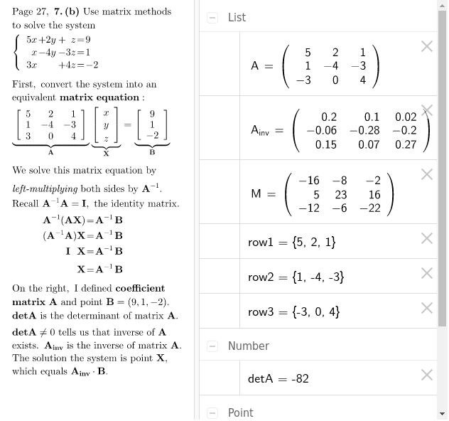
With the foundational components in place, we can now precisely define the matrix equation. The most common and canonical form of a matrix equation is:

Ax = b

Let’s break down each component:

The Core Components: A, x, and b Explained

• A (Coefficient Matrix): This is typically a square matrix (number of rows equals number of columns), but can also be rectangular. It contains the coefficients of the variables in a system of linear equations. In a broader sense, A represents a linear transformation or a set of relationships.

• x (Variable Vector): This is a column vector containing the unknown variables we are trying to solve for. These are the values we want to determine.

• b (Constant Vector): This is also a column vector, representing the known outcomes or constants of the system.

Consider a simple system of two linear equations:

2x_1 + 3x_2 = 8

4x_1 + 9x_2 = 20

This system can be rewritten in matrix form as Ax = b:

[ 2  3 ] [ x_1 ] = [ 8  ]

[ 4  9 ] [ x_2 ] = [ 20 ]

Here, A is the 2×2 coefficient matrix, x is the 2×1 variable vector, and b is the 2×1 constant vector. The goal of solving the matrix equation is to find the values in vector x that satisfy the given relationships.

Visualizing the Transformation: Geometric Interpretation

Beyond simply representing a system of equations, Ax = b has a powerful geometric interpretation, especially relevant in computer graphics and physics. The matrix A can be viewed as an operator that transforms the vector x from one space to another, resulting in the vector b.

For instance, if x represents a point in 2D space, and A is a rotation matrix, then Ax will be the new coordinates of that point after it has been rotated. If A is a scaling matrix, Ax will represent the scaled point. This transformation perspective is crucial for understanding how objects are manipulated in 3D environments, how images are processed, and how data points are re-projected in dimensionality reduction techniques like Principal Component Analysis (PCA).

Solving for the Unknown: Direct and Iterative Methods

Solving Ax = b for x is akin to finding the inverse of A and multiplying it by b (i.e., x = A⁻¹b), but directly computing the inverse A⁻¹ can be computationally intensive and unstable for large matrices. Therefore, various methods are employed:

• Direct Methods: These methods aim to find an exact solution in a finite number of steps. Examples include Gaussian Elimination, LU Decomposition, and Cholesky Decomposition. These are generally preferred for smaller, dense matrices where high precision is required.

• Iterative Methods: These methods start with an initial guess for x and then successively refine it through repeated calculations until a satisfactory level of accuracy is achieved. Examples include Jacobi, Gauss-Seidel, and Conjugate Gradient methods. Iterative methods are often more suitable for large, sparse matrices (matrices with many zero elements), which are common in scientific computing and machine learning.

The choice of method depends on the characteristics of the matrix A (size, sparsity, condition number) and the required precision.

Why Matrix Equations Matter in Technology

The power and versatility of matrix equations make them indispensable across a vast spectrum of technological applications. They provide an elegant and efficient way to model, analyze, and solve complex problems that underpin much of our digital world.

Computer Graphics and Game Development: Rendering the Digital World

Every 3D object you see on a screen, every animation, and every virtual world is meticulously constructed and manipulated using matrix equations.

• Transformations: Rotation, scaling, translation, and projection of 3D objects are all performed using transformation matrices. Multiplying a vertex vector by a transformation matrix applies the desired change.

• Camera Views: Defining what the “camera” sees involves view and projection matrices that transform 3D world coordinates into 2D screen coordinates.

• Lighting and Shading: Sophisticated lighting models often involve matrix operations to calculate how light interacts with surfaces.

Without matrix equations, the rich visual experiences of modern games, CAD software, and virtual reality would be impossible.

Machine Learning and Artificial Intelligence: The Brains Behind the Bots

Matrix equations are the bedrock of almost every machine learning algorithm, from simple linear regression to complex deep neural networks.

• Linear Regression: The core of finding the “best fit” line or plane involves solving Ax = b to determine the coefficients that minimize prediction errors.

• Neural Networks: Each layer in a neural network performs a matrix multiplication (weights * inputs) followed by an activation function. Training a neural network involves adjusting these weight matrices through backpropagation, an optimization process heavily reliant on matrix calculus.

• Dimensionality Reduction: Techniques like PCA use eigenvalue decomposition (a concept derived from matrix equations) to find principal components that capture the most variance in high-dimensional data, making it easier to analyze and visualize.

• Natural Language Processing: Word embeddings (vector representations of words) and transformer models (which power large language models like GPT) rely heavily on matrix operations for processing and understanding textual data.

Data Science and Analytics: Uncovering Insights from Raw Data

In data science, datasets are frequently represented as matrices, making matrix equations a natural tool for analysis.

• Statistical Analysis: Covariance matrices, correlation matrices, and various statistical models are built upon matrix algebra.

• Recommender Systems: Collaborative filtering algorithms, which suggest products or content based on user preferences, often model user-item interactions as matrices and use techniques like singular value decomposition (SVD) to find underlying patterns.

• Optimization Problems: Many data science problems, such as finding optimal parameters for a model or allocating resources, can be formulated and solved as matrix equations or systems involving matrices.

Engineering Simulations and Scientific Computing: Modeling Complex Systems

From designing aircraft to simulating climate change, engineering and scientific disciplines rely heavily on numerical methods powered by matrix equations.

• Finite Element Analysis (FEA): Used to simulate the behavior of structures under stress, heat, or fluid flow, FEA discretizes complex geometries into smaller elements, leading to large systems of linear equations that are solved using matrix methods.

• Computational Fluid Dynamics (CFD): Simulating fluid movement, such as airflow over a wing or blood flow in arteries, involves solving Navier-Stokes equations, which are often discretized and solved as large matrix equations.

• Quantum Mechanics: Many problems in quantum physics involve solving eigenvalue problems for matrices representing operators.

Beyond the Basics: Advanced Concepts and Applications

The utility of matrix equations extends into more advanced concepts, which further expand their power in tech.

Inverse Matrices and Determinants: Unlocking Solutions

The determinant is a scalar value that can be computed from the elements of a square matrix. It provides crucial information about the matrix, such as whether a unique solution exists for Ax = b. If the determinant is zero, the matrix is singular, and a unique solution does not exist.

The inverse matrix A⁻¹ is a matrix that, when multiplied by A, yields the identity matrix (a square matrix with ones on the main diagonal and zeros elsewhere). If A⁻¹ exists, then the solution to Ax = b can be directly found as x = A⁻¹b. While computationally expensive for large matrices, the concept of an inverse is theoretically vital.

Eigenvalues and Eigenvectors: Understanding System Dynamics

Eigenvalues and eigenvectors are special scalar-vector pairs that describe how a linear transformation affects certain vectors. When a matrix A acts on an eigenvector v, it only scales the vector (by the eigenvalue λ) without changing its direction: Av = λv.

This concept is profoundly important:

• In PCA, eigenvectors represent the principal components (directions of maximum variance) in a dataset.

• In quantum mechanics, eigenvectors represent possible states of a system, and eigenvalues represent observable quantities.

• In control systems, eigenvalues determine the stability and behavior of a system over time.

Practical Implementations: Libraries and Frameworks (e.g., NumPy, TensorFlow)

While the mathematical theory is crucial, software developers and data scientists rarely solve matrix equations from scratch. Instead, they leverage powerful libraries and frameworks that provide highly optimized implementations of matrix operations.

• NumPy (Python): The cornerstone of scientific computing in Python, NumPy provides robust support for multi-dimensional arrays (matrices) and a comprehensive suite of linear algebra functions.

• SciPy (Python): Builds on NumPy, offering more advanced linear algebra routines, including solvers for large sparse matrix equations.

• MATLAB: A widely used proprietary environment for numerical computation, known for its strong matrix manipulation capabilities.

• TensorFlow/PyTorch: These deep learning frameworks are built from the ground up to handle massive matrix and tensor (higher-dimensional matrices) operations efficiently, often leveraging GPU acceleration.

These tools abstract away the complexity of the underlying algorithms, allowing practitioners to focus on modeling and solving problems rather than implementing low-level matrix math.

Conclusion: The Unsung Hero of Modern Tech

The matrix equation, Ax = b, might appear simple on the surface, but its implications and applications are anything but. It is a unifying concept that provides a consistent language and methodology for solving an incredibly diverse range of problems across the technological spectrum. From rendering photorealistic scenes and empowering intelligent machines to sifting through vast oceans of data and simulating complex physical phenomena, matrix equations are the unsung heroes working tirelessly behind the scenes.

For anyone venturing into fields like computer science, data science, AI, or engineering, a solid grasp of what the matrix equation represents, how it functions, and why it’s so powerful is not just beneficial—it’s absolutely essential. It provides a foundational understanding that bridges pure mathematics with the innovative frontiers of modern technology. As technology continues to advance, the role of matrix equations will only grow, cementing their status as an indispensable tool for future innovation.

aViewFromTheCave is a participant in the Amazon Services LLC Associates Program, an affiliate advertising program designed to provide a means for sites to earn advertising fees by advertising and linking to Amazon.com. Amazon, the Amazon logo, AmazonSupply, and the AmazonSupply logo are trademarks of Amazon.com, Inc. or its affiliates. As an Amazon Associate we earn affiliate commissions from qualifying purchases.