The kinematic equations are a cornerstone of classical mechanics, providing a powerful framework for understanding and predicting the motion of objects. These equations, derived from fundamental principles of physics, are not just abstract mathematical constructs; they are essential tools in a wide range of technological applications, from the design of autonomous vehicles and robotics to the simulation of complex physical phenomena in engineering and scientific research. In the realm of technology, grasping the kinematic equations unlocks deeper insights into how systems move, interact, and operate in the physical world.
The Foundations of Motion: Understanding Velocity and Acceleration
At its core, kinematics is the study of motion without considering the forces that cause it. It focuses purely on the geometric aspects of movement: position, displacement, velocity, and acceleration. To truly understand kinematic equations, we must first establish a clear understanding of these fundamental concepts.

Displacement and Position
Position refers to the location of an object in space at a specific point in time. It’s usually represented as a vector, indicating both distance and direction from a chosen origin. Displacement, on the other hand, is the change in an object’s position over a period. It’s also a vector quantity, meaning it has both magnitude and direction. For instance, if a robot moves 5 meters east and then 2 meters west, its total displacement is 3 meters east, even though its total distance traveled is 7 meters. This distinction is crucial; kinematic equations deal with displacement, not necessarily the path taken.
Velocity: The Rate of Change of Position
Velocity describes how quickly an object’s position is changing. It’s a vector quantity, encompassing both speed (the magnitude of velocity) and direction. Average velocity is calculated by dividing the total displacement by the total time taken.
$$ text{Average Velocity} = frac{text{Displacement}}{text{Time Interval}} = frac{Delta x}{Delta t} $$
where $Delta x$ is the displacement and $Delta t$ is the time interval.
Instantaneous velocity is the velocity of an object at a single, specific moment in time. It’s essentially the average velocity as the time interval approaches zero. In many technological applications, such as controlling the speed of a drone or a conveyor belt, understanding and calculating instantaneous velocity is paramount for precise operation.
Acceleration: The Rate of Change of Velocity
Acceleration is the rate at which an object’s velocity changes. Like velocity, it’s a vector quantity and can involve changes in speed, direction, or both. Average acceleration is calculated by dividing the change in velocity by the time interval over which that change occurs.
$$ text{Average Acceleration} = frac{text{Change in Velocity}}{text{Time Interval}} = frac{Delta v}{Delta t} $$
where $Delta v$ is the change in velocity.
Instantaneous acceleration is the acceleration at a specific moment in time. This is particularly important in systems that require dynamic adjustments, such as the braking system of an autonomous car or the torque control in a robotic arm. If an object is moving at a constant velocity, its acceleration is zero. Any change in velocity, whether speeding up, slowing down, or changing direction, implies acceleration.
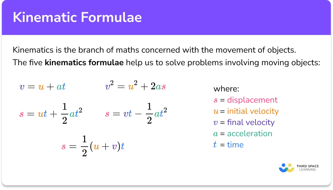
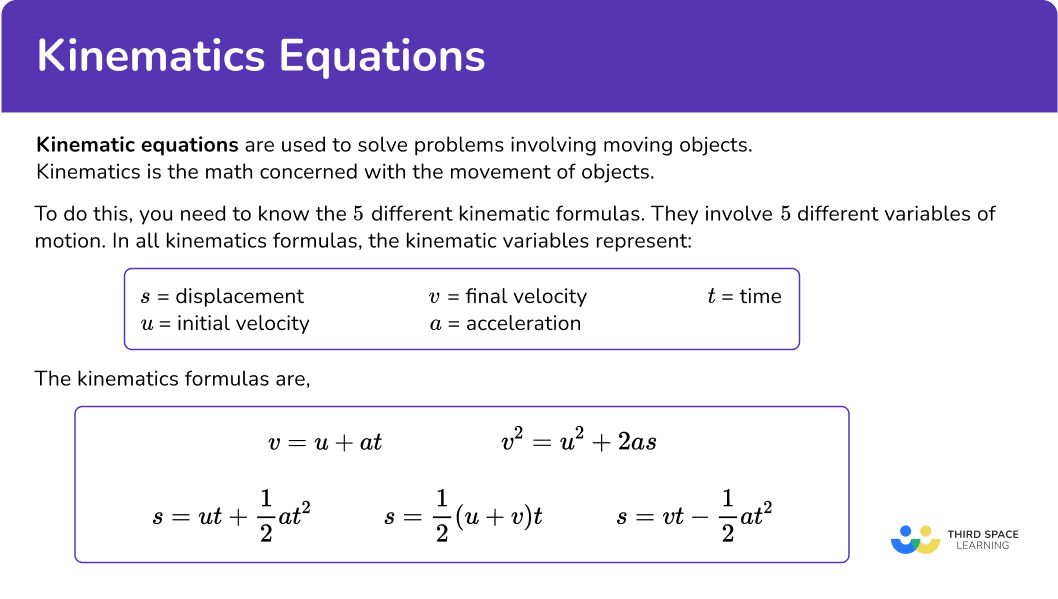
The Five Core Kinematic Equations for Constant Acceleration
The power of kinematics lies in its ability to describe motion using a set of elegant mathematical relationships. When the acceleration of an object is constant, a particularly useful set of five equations, often referred to as the “kinematic equations” or “SUVAT equations” (where SUVAT stands for displacement, initial velocity, final velocity, acceleration, and time), can be applied. These equations allow us to solve for any unknown variable if we know three other variables.
Let’s define the variables we’ll be using:
- $v_f$: final velocity
- $v_i$: initial velocity
- $a$: acceleration (assumed constant)
- $Delta x$: displacement
- $t$: time interval
Equation 1: The Velocity-Time Relation
This equation relates final velocity, initial velocity, acceleration, and time. It’s derived directly from the definition of constant acceleration.
$$ vf = vi + at $$
This equation is fundamental for predicting the velocity of an object at any given time, given its initial velocity and constant acceleration. For example, in designing a robotic arm that needs to move a certain distance in a specific time, engineers might use this equation to determine the required acceleration profile. If a robot’s gripper starts from rest ($vi = 0$) and accelerates at $2 , text{m/s}^2$ for $3$ seconds, its final velocity will be $vf = 0 + (2 , text{m/s}^2)(3 , text{s}) = 6 , text{m/s}$.
Equation 2: The Displacement-Time Relation (with initial velocity)
This equation relates displacement, initial velocity, acceleration, and time. It’s a direct consequence of integrating the velocity equation over time.
$$ Delta x = v_i t + frac{1}{2} at^2 $$
This equation is incredibly useful for determining how far an object will travel under constant acceleration. In applications like projectile motion simulations for drones or trajectory planning for autonomous vehicles, this equation helps predict the path and reach of an object. If a delivery drone starts with an initial downward velocity of $5 , text{m/s}$ and accelerates downwards at $9.8 , text{m/s}^2$ due to gravity for $2$ seconds, its displacement will be $Delta x = (5 , text{m/s})(2 , text{s}) + frac{1}{2} (9.8 , text{m/s}^2)(2 , text{s})^2 = 10 , text{m} + 19.6 , text{m} = 29.6 , text{m}$ downwards.
Equation 3: The Displacement-Velocity Relation (without time)
This equation relates displacement, initial velocity, final velocity, and acceleration. It’s particularly handy when the time interval is unknown or not relevant to the problem at hand. It’s derived by eliminating time ($t$) from the first two equations.
$$ vf^2 = vi^2 + 2a Delta x $$
This equation is frequently used in scenarios where you need to know the speed of an object after it has traveled a certain distance or when you want to determine the distance required to reach a specific speed. Consider the design of safety systems in autonomous vehicles. To ensure a vehicle can stop safely, engineers need to calculate the braking distance. If a car is traveling at $30 , text{m/s}$ and the maximum safe deceleration is $-8 , text{m/s}^2$, the stopping distance can be calculated: $(0 , text{m/s})^2 = (30 , text{m/s})^2 + 2(-8 , text{m/s}^2) Delta x$. Solving for $Delta x$ gives approximately $56.25$ meters, a critical piece of information for programming emergency braking.
Equation 4: The Displacement-Time Relation (with average velocity)
This equation relates displacement, average velocity, and time. It’s a direct application of the definition of average velocity, assuming constant acceleration.
$$ Delta x = frac{vi + vf}{2} t $$
This equation offers a simplified way to calculate displacement when both initial and final velocities are known, along with the time taken. It highlights that under constant acceleration, the displacement is equal to the average velocity multiplied by the time. In simulations for game development or virtual reality environments, this equation can be used to smoothly animate the movement of objects. If a character in a game starts with a velocity of $10 , text{m/s}$ and ends with $20 , text{m/s}$ after $5$ seconds, its displacement is $Delta x = frac{10 , text{m/s} + 20 , text{m/s}}{2} (5 , text{s}) = (15 , text{m/s})(5 , text{s}) = 75 , text{m}$.
Equation 5: The Velocity-Time Relation (with displacement)
This equation relates final velocity, initial velocity, acceleration, and displacement. It’s derived by manipulating the displacement-time equation to solve for time and then substituting that into the velocity-time equation, or by directly solving for $v_f$ from the third equation.
$$ vf = sqrt{vi^2 + 2a Delta x} $$
While mathematically derivable from the others, this form explicitly shows the final velocity based on initial velocity, acceleration, and the distance traveled. It’s useful when time is not a factor but you need to know the resultant speed after a certain movement. For instance, in designing the landing gear for an aircraft, engineers would use principles related to this equation to ensure the landing gear can withstand the impact velocity after a certain drop distance.
Applications in Modern Technology
The seemingly simple kinematic equations are the bedrock upon which much of modern technology is built. Their ability to precisely model and predict motion underpins the functionality of countless devices and systems.
Robotics and Automation
In the field of robotics, kinematic equations are fundamental to controlling the movement of robotic arms, mobile robots, and automated machinery.
Path Planning and Control
Robots need to navigate complex environments and perform intricate tasks. Path planning algorithms rely heavily on kinematic equations to calculate the required sequences of movements. For a robotic arm to pick up an object, its joints must move in a coordinated manner. Kinematic equations help determine the precise angles and velocities each joint needs to achieve to move the end-effector (the robot’s hand) to the target location. Control systems then use these calculated parameters to send signals to the robot’s motors, ensuring smooth and accurate motion. This involves calculating desired velocities and accelerations based on the target path and the robot’s current state.
Autonomous Navigation
Autonomous vehicles, from self-driving cars to delivery drones, are sophisticated applications of kinematic principles. When an autonomous vehicle needs to change lanes, brake, or accelerate, its onboard computer uses kinematic equations to predict its trajectory and the trajectory of other objects in its vicinity.
Sensor fusion often combines data from various sensors (LiDAR, radar, cameras) to create a comprehensive understanding of the vehicle’s environment. Kinematic models then take this information and predict how the vehicle will move. For example, if a self-driving car detects an obstacle ahead, it uses kinematic equations to determine the necessary braking force and distance to stop safely, or if it can safely swerve. The prediction of future positions and velocities of both the vehicle and potential hazards is entirely dependent on these equations.
Simulation and Virtual Environments
The development of realistic simulations for training, entertainment, and design relies heavily on accurately modeling physical phenomena, including motion.
Game Development
In video games, players expect characters and objects to move in a believable way. Game engines use kinematic equations to simulate everything from character jumps and projectile trajectories to the physics of collisions. When a player character jumps, the engine calculates the parabolic path of their movement using equations of motion under gravity. Projectiles fired by enemies or weapons follow similar kinematic paths. The more accurate the kinematic simulation, the more immersive and satisfying the gaming experience.
Engineering Design and Virtual Prototyping
Engineers use kinematic simulations to test designs before building physical prototypes. This is particularly crucial in industries like automotive, aerospace, and manufacturing. For example, an engineer designing a new car suspension system can use kinematic simulations to analyze how the wheels will move over different terrains and how the suspension will react. This allows them to identify potential issues and optimize the design without the cost and time involved in building multiple physical prototypes. Similarly, for designing complex machinery like factory automation systems, kinematic simulations ensure that moving parts will not collide and that the overall operation is efficient.
Human-Computer Interaction and Motion Tracking
Kinematic principles are also vital in how we interact with technology through movement.
Motion Capture Technology
Motion capture technology, used extensively in film, animation, and sports analysis, relies on tracking the movement of markers placed on a subject’s body. Kinematic equations are then used to translate these marker positions into realistic skeletal animations. The system tracks the spatial coordinates of the markers over time, and from this, it can infer velocities, accelerations, and the overall kinematics of the motion, allowing for the creation of highly realistic digital characters or the analysis of athletic performance.
Wearable Technology and Gesture Recognition
Wearable devices, such as smartwatches and fitness trackers, use accelerometers and gyroscopes to track user activity. The raw data from these sensors is processed using kinematic principles to determine steps taken, distance covered, and even the type of activity being performed. Furthermore, gesture recognition systems in smartphones and other devices use kinematic analysis of sensor data to interpret hand movements or body gestures, enabling new ways of interacting with technology without direct touch input.
Beyond Constant Acceleration: Introducing Calculus
While the five core kinematic equations are incredibly powerful, they are limited to situations with constant acceleration. In many real-world technological applications, acceleration is not constant; it can vary with time, position, or velocity. To accurately model such complex motions, we must turn to the tools of calculus.
Velocity as the Integral of Acceleration
If acceleration is not constant, we can express velocity as the integral of acceleration with respect to time:
$$ v(t) = vi + int{0}^{t} a(tau) , dtau $$
This equation signifies that the change in velocity over a time interval is the accumulated effect of acceleration over that same interval. For instance, in designing an advanced flight control system for an aircraft, the thrust of the engines and atmospheric conditions can lead to non-uniform acceleration. Engineers would use integration to calculate the aircraft’s velocity at any given moment.
Displacement as the Integral of Velocity
Similarly, displacement can be found by integrating velocity with respect to time:
$$ Delta x(t) = int_{0}^{t} v(tau) , dtau $$
This equation allows us to calculate the total distance traveled or the final position of an object when its velocity is continuously changing. In optimizing the performance of electric vehicles, understanding how battery power translates into varying acceleration and thus varying velocity over a drive is crucial for accurate range prediction and energy management.
Acceleration as the Derivative of Velocity
Conversely, if we know the velocity function, we can find the acceleration by taking its derivative:
$$ a(t) = frac{dv}{dt} $$
This relationship is fundamental for analyzing and controlling systems where acceleration is a direct consequence of velocity. For example, in developing advanced suspension systems for vehicles, the forces acting on the suspension are often dependent on the velocity of the vehicle, leading to a non-constant acceleration profile that can be analyzed using calculus.
By employing calculus, the principles of kinematics can be extended to model a far wider range of dynamic systems, from the complex movements of celestial bodies to the intricate mechanics of microscopic machines, further solidifying their indispensable role in technological advancement.
Conclusion: The Ubiquitous Power of Kinematic Equations
The kinematic equations, whether in their simple constant-acceleration form or their advanced calculus-based extensions, are fundamental pillars of physics and technology. They provide the language and the tools to describe, understand, and predict motion. From the sophisticated algorithms guiding autonomous vehicles and the precise movements of industrial robots to the immersive worlds of video games and the detailed analysis of human motion, these equations are quietly at work, enabling innovation and shaping the technological landscape. As technology continues to evolve, a solid grasp of kinematics will remain an invaluable asset for anyone seeking to understand, design, or improve the systems that move our world.
aViewFromTheCave is a participant in the Amazon Services LLC Associates Program, an affiliate advertising program designed to provide a means for sites to earn advertising fees by advertising and linking to Amazon.com. Amazon, the Amazon logo, AmazonSupply, and the AmazonSupply logo are trademarks of Amazon.com, Inc. or its affiliates. As an Amazon Associate we earn affiliate commissions from qualifying purchases.