What is Excel VLOOKUP?

Excel’s VLOOKUP function is a cornerstone of data analysis and manipulation within the spreadsheet software. For anyone working with large datasets, needing to connect information across different tables, or seeking to automate repetitive data retrieval tasks, understanding VLOOKUP is not just beneficial – it’s essential. This powerful function allows you to search for a specific value in the first column of a table and return a corresponding value from a different column in the same row. Imagine it as a sophisticated search engine built directly into your spreadsheet, capable of fetching precisely the piece of information you need, exactly when you need it.

At its core, VLOOKUP is designed to tackle the common problem of fragmented data. Often, critical information is spread across multiple tables or worksheets, making it difficult to compile a complete picture. VLOOKUP bridges this gap, enabling you to look up a unique identifier (like a product ID, employee number, or customer name) in one table and pull associated details (like product price, department, or contact information) from another. This not only saves an immense amount of manual effort but also dramatically reduces the risk of human error that can creep into copy-pasting operations.

The versatility of VLOOKUP extends across various professional domains. In finance, it can be used to match transaction IDs with customer records. In sales, it can pull product details from an inventory list based on a sales order. In human resources, it can fetch employee benefits information from a central HR database using an employee ID. Even in academic research, VLOOKUP can help correlate student IDs with their respective performance metrics. The ability to dynamically link and retrieve data makes it an indispensable tool for anyone looking to gain deeper insights from their spreadsheets.

The Anatomy of a VLOOKUP Formula

To truly grasp the power of VLOOKUP, it’s crucial to understand its constituent parts. The function is constructed with four arguments, each playing a specific role in defining the search and retrieval process. Mastering these arguments is the key to unlocking VLOOKUP’s full potential and avoiding common pitfalls.

The Four Essential Arguments

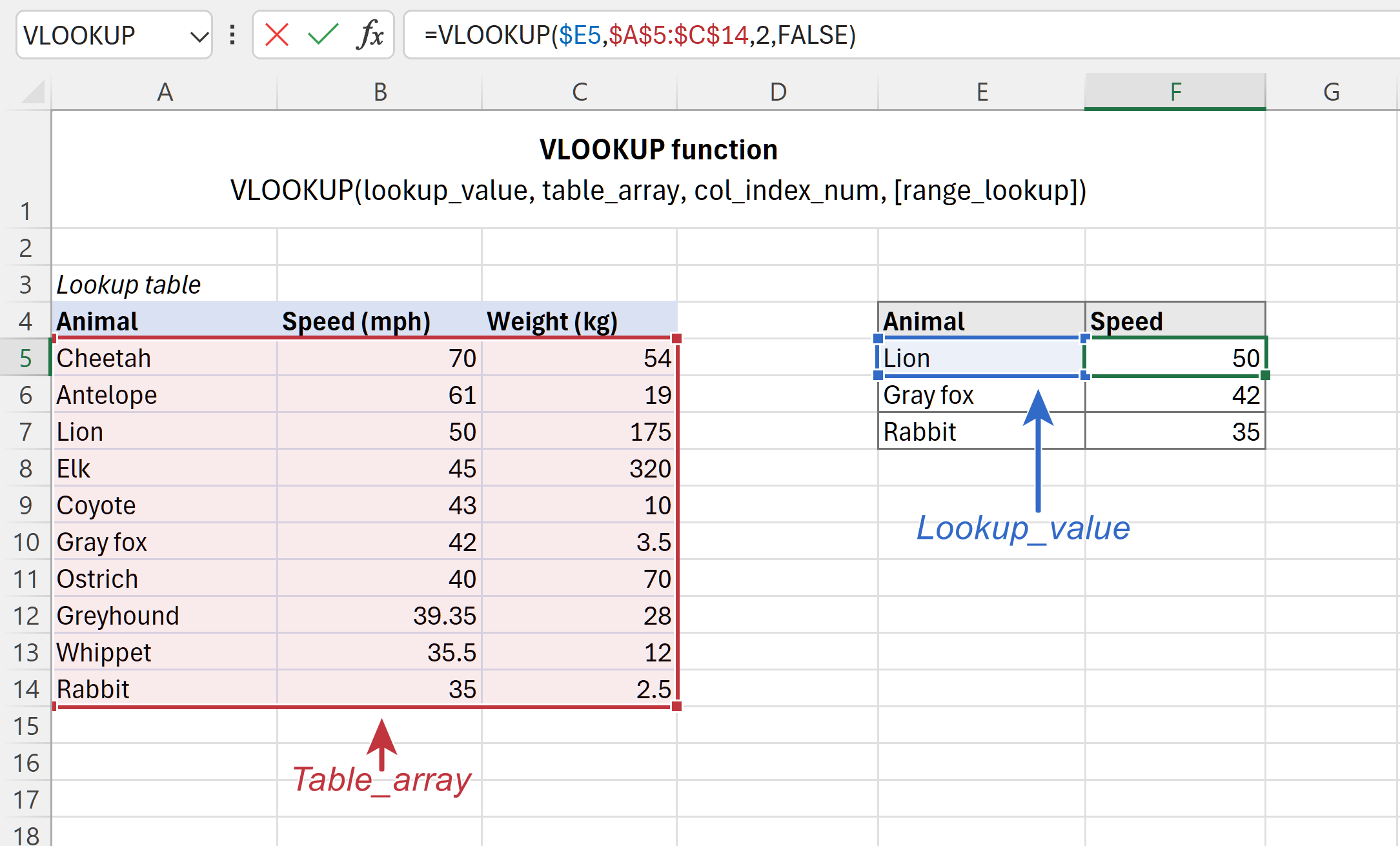
The syntax for VLOOKUP is as follows: =VLOOKUP(lookup_value, table_array, col_index_num, [range_lookup]). Let’s break down each of these components:

lookup_value: What You’re Searching For

This is the value that VLOOKUP will search for in the first column of your specified table. It’s the identifier you want to find. This could be a specific number, a piece of text, a date, or even a cell reference containing the value you’re looking for. For example, if you’re trying to find the price of a specific product, the lookup_value would be the product’s unique ID or name.

table_array: Where You’re Searching

This refers to the range of cells that contains the data you want to search within. Importantly, the lookup_value must be present in the first column of this table_array. The table_array can span multiple columns and rows. It’s common practice to use absolute references (e.g., $A$1:$D$100) for the table_array when copying the formula down, ensuring that the search range remains fixed. This prevents the range from shifting and causing errors.

col_index_num: Which Column to Pull Data From

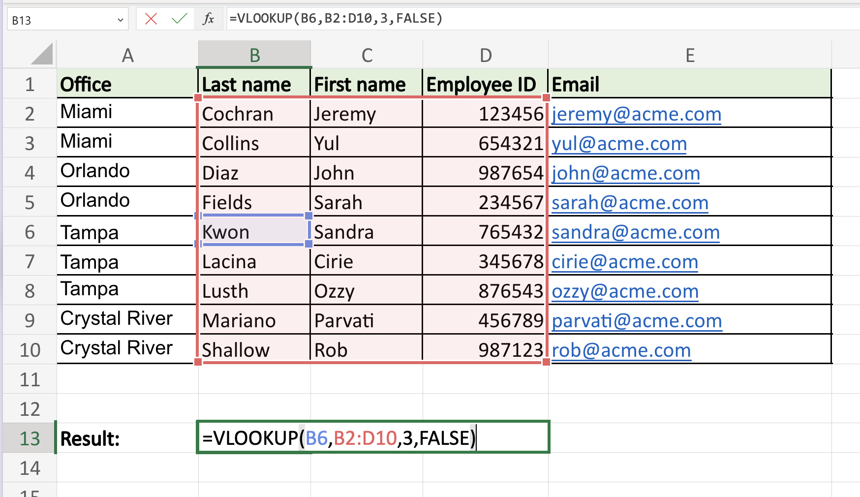
Once VLOOKUP finds the lookup_value in the first column of the table_array, it needs to know which column to return the corresponding data from. The col_index_num is a number representing the column within the table_array that contains the information you want to retrieve. The first column of the table_array is considered column 1, the second is column 2, and so on. For instance, if your table_array is A1:D10 and you want to retrieve data from the third column (column C), your col_index_num would be 3.

[range_lookup]: Exact Match or Approximate Match

This is a crucial argument, and it can be either TRUE (or omitted) for an approximate match, or FALSE for an exact match.

• FALSE (Exact Match): This is the most common and generally recommended setting for most use cases. When range_lookup is set to FALSE, VLOOKUP will only return a value if it finds an exact match for the lookup_value in the first column of the table_array. If no exact match is found, it will return a #N/A error. This is ideal for situations where you need precise data correlation, such as looking up a specific customer’s order number or a product’s exact price.

• TRUE (Approximate Match): When range_lookup is set to TRUE (or if you omit this argument, as TRUE is the default), VLOOKUP will search for an approximate match. This means that if an exact match isn’t found, VLOOKUP will find the largest value that is less than or equal to the lookup_value. For this to work correctly, the first column of your table_array must be sorted in ascending order. Approximate matches are typically used for scenarios like determining tax brackets, grading scales, or commission tiers based on sales figures. For example, if you have a table with sales ranges (e.g., 0-1000, 1001-5000, 5001+) and corresponding commission rates, you could use TRUE to find the correct commission rate for any given sales amount.

Understanding the distinction between TRUE and FALSE is paramount to avoiding incorrect data retrieval and ensuring the reliability of your spreadsheet analyses.

Practical Applications of VLOOKUP

The theoretical understanding of VLOOKUP’s arguments is only the first step. Its true value is realized when applied to real-world scenarios. VLOOKUP’s ability to automate data retrieval and integration makes it a workhorse for a multitude of tasks, saving users significant time and effort.

Scenario 1: Merging Customer Data

Imagine you have two spreadsheets. The first contains a list of recent sales transactions, including customer IDs. The second spreadsheet contains a comprehensive customer database with customer IDs, names, addresses, and contact information. You want to add the customer names and addresses directly to your sales transaction sheet.

Instead of manually searching for each customer ID in the second sheet and copying their details, you can use VLOOKUP.

Formula Example:
Assuming your sales transactions are in Sheet1 with customer IDs in column A, and your customer database is in Sheet2 with customer IDs in column A, customer names in column B, and addresses in column C. To pull the customer name into Sheet1, in a new column (say, column B), you would use:

=VLOOKUP(A2, Sheet2!$A$2:$C$1000, 2, FALSE)

Here:

• A2 is the lookup_value (the customer ID in the current sales transaction row).
• Sheet2!$A$2:$C$1000 is the table_array (the customer database, with absolute references to keep the range fixed).
• 2 is the col_index_num (the second column in the table_array, which is the customer name).
• FALSE ensures an exact match for the customer ID.

You would then drag this formula down to apply it to all sales transactions. To pull the address, you would use a similar formula with col_index_num set to 3.

Scenario 2: Populating Product Information

Consider an e-commerce business that has an inventory list with product IDs, names, descriptions, and prices. When new orders come in, they might only contain product IDs. You need to quickly populate the order details with the corresponding product names and prices.

Formula Example:
Let’s say your inventory is in Sheet1, with Product IDs in column A, Product Names in column B, and Prices in column C. Your new order details are in Sheet2, with Product IDs in column A. To get the Product Name into Sheet2, column B:

=VLOOKUP(A2, Sheet1!$A$2:$C$500, 2, FALSE)

And to get the Price into Sheet2, column C:

=VLOOKUP(A2, Sheet1!$A$2:$C$500, 3, FALSE)

Again, A2 is the lookup_value (the product ID), Sheet1!$A$2:$C$500 is the table_array, 2 and 3 are the respective col_index_num for name and price, and FALSE ensures an exact product ID match.

Scenario 3: Creating Grading Scales

In an educational setting, you might have a list of student scores and a separate table defining the grading scale (e.g., score ranges and corresponding letter grades). VLOOKUP can automate the assignment of grades.

Formula Example:
Suppose your student scores are in Sheet1, column A. Your grading scale is in Sheet2, with the lower bound of each score range in column A (e.g., 0, 60, 70, 80, 90) and the corresponding letter grades (F, D, C, B, A) in column B. To assign grades in Sheet1, column B:

=VLOOKUP(A2, Sheet2!$A$2:$B$6, 2, TRUE)

Here:

• A2 is the lookup_value (the student’s score).
• Sheet2!$A$2:$B$6 is the table_array (the grading scale, ensure column A is sorted in ascending order).
• 2 is the col_index_num (the letter grade).
• TRUE is used for an approximate match. This will find the largest score in Sheet2’s column A that is less than or equal to the student’s score in A2, and return the corresponding grade from column B.

These examples highlight how VLOOKUP streamlines processes, reduces manual effort, and improves accuracy across diverse data-intensive tasks.

Limitations and Advanced Alternatives

While VLOOKUP is a powerful and widely used function, it does come with certain limitations that users should be aware of. Recognizing these constraints can help you choose the right tool for the job and avoid potential frustrations. Fortunately, Excel offers more advanced functions that overcome these limitations.

Understanding VLOOKUP’s Constraints

1. Search Direction: VLOOKUP can only search for the lookup_value in the first column of the table_array and return data from columns to the right of that first column. It cannot look up a value in the second column and return data from the first, nor can it look up in the last column and return data from earlier columns. This inherent directional limitation can be a significant constraint when your data isn’t structured in the ideal left-to-right lookup format.

2. Column Insertion/Deletion: If you insert or delete columns within your table_array after you’ve set up your VLOOKUP formula, the col_index_num will no longer point to the correct column. For example, if you had a formula using col_index_num = 3 and you insert a new column before the original third column, the original third column now becomes the fourth column, and your VLOOKUP will pull data from the wrong place, leading to errors. This makes formulas brittle and prone to breaking when the underlying data structure changes.

3. Performance Issues with Large Datasets: While VLOOKUP is generally efficient, in extremely large datasets (hundreds of thousands or millions of rows), performance can degrade. Repeatedly calculating VLOOKUP formulas across many rows can slow down your workbook significantly, impacting user experience and workflow.

4. #N/A Errors: As mentioned, when an exact match isn’t found (with range_lookup = FALSE), VLOOKUP returns a #N/A error. While this is informative, it can clutter your results and may require additional error-handling formulas (like IFERROR) to manage.

Introducing XLOOKUP and INDEX/MATCH

To address these limitations, Excel has introduced more flexible and robust lookup functions.

XLOOKUP: The Modern Successor

Introduced in newer versions of Excel (Microsoft 365 and Excel 2021), XLOOKUP is designed to supersede VLOOKUP and HLOOKUP. It’s far more versatile and user-friendly.

Key Advantages of XLOOKUP:

• Bidirectional Lookup: XLOOKUP can look up a value in any column and return data from any column, regardless of their relative positions.
• Easier Syntax: The arguments are more intuitive. It separates the column to search in from the column to return from. The syntax is: =XLOOKUP(lookup_value, lookup_array, return_array, [if_not_found], [match_mode], [search_mode]).
• Built-in Error Handling: The [if_not_found] argument allows you to specify what to return if the lookup_value is not found, eliminating the need for separate IFERROR functions.
• Column Insertion Robustness: Because XLOOKUP specifies distinct lookup and return arrays (columns), inserting or deleting columns within your data range does not break the formula, as long as the specified columns remain the same.
• Performance: Generally performs better with large datasets.

Example using XLOOKUP (equivalent to the customer data scenario):
=XLOOKUP(A2, Sheet2!$A$2:$A$1000, Sheet2!$B$2:$B$1000, "Customer Not Found")
Here, A2 is the lookup_value, Sheet2!$A$2:$A$1000 is the column to search in (customer IDs), and Sheet2!$B$2:$B$1000 is the column to return from (customer names). “Customer Not Found” handles the #N/A scenario.

INDEX and MATCH: The Flexible Power Duo

Before XLOOKUP was available, the combination of INDEX and MATCH was the preferred method for overcoming VLOOKUP’s limitations. While the syntax is more complex, it offers unparalleled flexibility.

• MATCH Function: Finds the position of a lookup_value within a row or column. =MATCH(lookup_value, lookup_array, [match_type]).
• INDEX Function: Returns a value from a specific row and column within a given range. =INDEX(array, row_num, [column_num]).

By nesting MATCH within INDEX, you can achieve the same results as VLOOKUP and more.

Example using INDEX/MATCH (equivalent to customer data scenario):
=INDEX(Sheet2!$B$2:$B$1000, MATCH(A2, Sheet2!$A$2:$A$1000, 0))

Here:

• Sheet2!$B$2:$B$1000 is the array from which to return the value (customer names).
• MATCH(A2, Sheet2!$A$2:$A$1000, 0) finds the row number of the lookup_value (A2) within the customer ID column (Sheet2!$A$2:$A$1000). The 0 in MATCH signifies an exact match.

INDEX/MATCH is still a valuable technique to know, especially if you are working with older versions of Excel or need the granular control it offers.

In conclusion, while VLOOKUP remains a foundational function in Excel, understanding its limitations and the advantages of XLOOKUP and INDEX/MATCH empowers users to perform even more sophisticated and robust data analysis. As data becomes increasingly complex and voluminous, these advanced lookup techniques are indispensable for efficient and accurate spreadsheet management.

aViewFromTheCave is a participant in the Amazon Services LLC Associates Program, an affiliate advertising program designed to provide a means for sites to earn advertising fees by advertising and linking to Amazon.com. Amazon, the Amazon logo, AmazonSupply, and the AmazonSupply logo are trademarks of Amazon.com, Inc. or its affiliates. As an Amazon Associate we earn affiliate commissions from qualifying purchases.