
In the realm of computer science and software engineering, the efficiency of data retrieval often dictates the performance of an entire application. As datasets grow in complexity and scale, the structures used to store and organize this information must evolve beyond simple linear lists. Among the most critical innovations in algorithmic efficiency is the AVL tree. Named after its Soviet inventors, Georgy Adelson-Velsky and Evgenii Landis, who introduced it in their 1962 paper, the AVL tree was the first “self-balancing” binary search tree ever devised. It remains a cornerstone of computer science education and a vital component in high-performance software systems.
Understanding the Fundamentals of AVL Trees
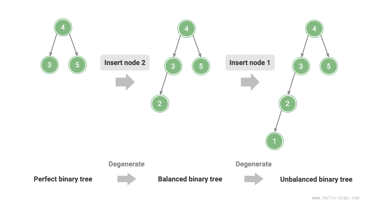
To understand why an AVL tree is necessary, one must first understand the limitations of a standard Binary Search Tree (BST). In a BST, each node has at most two children, and for any given node, all elements in the left subtree are smaller, while all elements in the right subtree are larger. When a BST is perfectly balanced, operations like searching, insertion, and deletion occur in logarithmic time—O(log n). However, the efficiency of a BST is highly dependent on the order in which data is inserted.
The Problem with Standard Binary Search Trees
The primary weakness of a basic BST is its susceptibility to becoming “skewed.” If data is inserted in sorted or nearly sorted order (e.g., 1, 2, 3, 4, 5), the tree degenerates into a structure that effectively functions as a linked list. In this “degenerate” state, the time complexity for finding an element reverts from O(log n) to O(n). For a database containing millions of records, this performance degradation is catastrophic. An AVL tree solves this by enforcing a strict structural constraint that ensures the tree remains balanced at all times, regardless of the input order.
Defining the Balance Factor
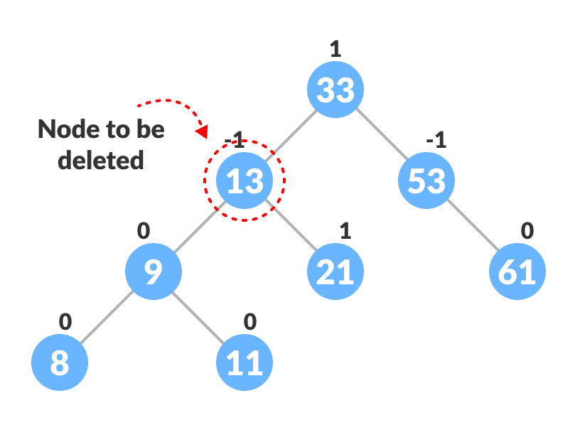
The “magic” of an AVL tree lies in its definition of balance. In an AVL tree, the heights of the two child subtrees of any node differ by at most one. This property is tracked through a metric known as the “Balance Factor.”
The Balance Factor (BF) of a node is calculated as:
BF = Height(Left Subtree) – Height(Right Subtree)
In an AVL tree, for every single node, the Balance Factor must be -1, 0, or 1. If at any point after an insertion or deletion the Balance Factor of a node becomes -2 or 2, the tree is considered “unbalanced,” and a rebalancing operation must be triggered immediately. By maintaining this property, the height of an AVL tree with $n$ nodes is always guaranteed to be proportional to log $n$, ensuring that search operations remain incredibly fast.
How AVL Trees Maintain Balance: The Four Rotations
The process of maintaining an AVL tree involves checking the balance factor of nodes following every modification. If a node becomes unbalanced, the algorithm performs a series of “rotations.” These rotations are algebraic rearrangements of the tree’s nodes that restore the height balance while preserving the binary search property (the relative order of the keys).
Single Rotations (Left and Right)
Single rotations are used when an imbalance is “linear”—meaning the heavy part of the tree is either entirely on the left or entirely on the right.
- Right Rotation (LL Rotation): This occurs when a node is added to the left child of a left child, causing a left-heavy imbalance. To fix this, the imbalanced node is rotated “down” to the right, and its left child is promoted to take its place.
- Left Rotation (RR Rotation): This is the mirror image of the right rotation. It occurs when a node is added to the right child of a right child. The imbalanced node is rotated “down” to the left, and its right child is promoted.
These operations are computationally inexpensive, involving only a few pointer reassignments, yet they significantly impact the overall depth of the tree.
Double Rotations (Left-Right and Right-Left)
Sometimes, an imbalance occurs in a “zigzag” pattern, where a single rotation is insufficient to restore balance. In these cases, a double rotation is required.
- Left-Right Rotation (LR Rotation): This happens when a node is inserted into the right subtree of a left child. The algorithm first performs a left rotation on the child node to transform the zigzag into a straight line (linear imbalance), followed by a right rotation on the parent node to restore total balance.
- Right-Left Rotation (RL Rotation): Conversely, this occurs when a node is inserted into the left subtree of a right child. A right rotation is performed on the child, followed by a left rotation on the parent.
While slightly more complex than single rotations, double rotations still occur in O(1) time, ensuring that the overhead of maintaining the tree does not negate its performance benefits.
Computational Efficiency and Performance Metrics
When evaluating data structures, software architects look at asymptotic complexity to predict how a system will scale. The AVL tree is optimized for scenarios where lookups are the most frequent operation.
Time Complexity Analysis
The most significant advantage of an AVL tree is its performance consistency. In a standard BST, the worst-case scenario is O(n). In an AVL tree, the worst-case scenario for search, insertion, and deletion is O(log n).
- Search: Because the tree is strictly balanced, the maximum path from the root to any leaf is roughly 1.44 * log n. This makes searching extremely predictable and fast.
- Insertion: Insertion requires a search to find the correct spot, followed by a balance factor check and potential rotations. While rotations add a small constant overhead, the overall complexity remains O(log n).
- Deletion: Deletion is the most complex operation. Removing a node may require multiple rotations as the “unbalance” can propagate up the tree toward the root. Even so, the total time remains logarithmic.
Space Complexity Considerations
From a memory perspective, an AVL tree requires O(n) space. Each node must store the data, pointers to two children, and an additional piece of information: the height of the node (or its balance factor). While this extra integer per node adds a small amount of memory overhead compared to a standard BST, the trade-off is almost always worth it given the massive gains in search speed and stability.
AVL Trees vs. Red-Black Trees: Choosing the Right Tool
In modern software development, AVL trees are often compared to Red-Black trees—another type of self-balancing BST used in libraries like the C++ STL (std::map) or Java’s TreeMap. While both provide O(log n) performance, they are optimized for different workloads.
When to Use AVL Trees
AVL trees are more “rigidly” balanced than Red-Black trees. A Red-Black tree allows for a bit more imbalance to reduce the frequency of rotations during insertions and deletions. Because AVL trees are more strictly balanced, they result in shorter average path lengths from the root to the leaves.
This makes AVL trees the superior choice for read-heavy workloads. If your application involves a dataset that is built once and searched millions of times, the extra effort spent balancing the tree during insertion is repaid every time a search is performed. Conversely, Red-Black trees are generally preferred for write-heavy workloads because they require fewer rotations on average during insertion and removal.
Real-World Applications in Software Engineering
Despite being decades old, the logic of the AVL tree is embedded in various modern technologies:
- Database Indexing: Many relational databases use variants of balanced trees to index primary keys, allowing for near-instantaneous record retrieval even in tables with billions of rows.
- Memory Management: Certain operating system kernels use balanced trees to keep track of allocated memory blocks, ensuring that the system can quickly find a free block of a specific size.
- High-Performance Computing: In any scenario where latency is critical—such as high-frequency trading or real-time simulation—the deterministic O(log n) lookup time of an AVL tree is invaluable.

Implementing AVL Trees in Modern Software Development
For developers looking to implement an AVL tree, the logic is typically encapsulated in a class or module to ensure the balancing properties are never violated by external code. Modern implementations often use recursion for insertion and deletion, as it allows the algorithm to check the balance factor of every ancestor node as the “recursion unwinds.”
When implementing, it is crucial to handle the height updates correctly. Each time a rotation occurs, the height of the affected nodes must be recalculated. Failure to do so will lead to incorrect balance factors, eventually causing the tree to lose its O(log n) guarantee.
Furthermore, in high-concurrency environments, developers must consider thread safety. Since rotations involve changing multiple pointers, an AVL tree must typically be protected by mutexes or implemented using non-blocking synchronization techniques to prevent data corruption when multiple threads attempt to modify the tree simultaneously.
In conclusion, the AVL tree represents a fundamental leap in data structure design. By introducing the concept of self-balancing through rotations, it provided a solution to the volatility of binary search trees. For tech professionals, understanding the mechanics of AVL trees—from balance factors to rotations—is more than an academic exercise; it is an insight into the principles of efficiency that power the modern digital world. Whether you are optimizing a database or building a custom search engine, the AVL tree remains one of the most elegant and effective tools in a programmer’s arsenal.
aViewFromTheCave is a participant in the Amazon Services LLC Associates Program, an affiliate advertising program designed to provide a means for sites to earn advertising fees by advertising and linking to Amazon.com. Amazon, the Amazon logo, AmazonSupply, and the AmazonSupply logo are trademarks of Amazon.com, Inc. or its affiliates. As an Amazon Associate we earn affiliate commissions from qualifying purchases.