How to Find the Function of a Graph

Understanding how to derive the mathematical function from a visual graph is a fundamental skill in numerous technical and scientific disciplines. Whether you’re a student grappling with algebra, an engineer analyzing sensor data, a data scientist building predictive models, or a researcher interpreting experimental results, the ability to translate a visual pattern into a precise mathematical equation is invaluable. This process bridges the gap between raw data visualization and actionable mathematical models, enabling deeper analysis, prediction, and communication.

In an increasingly data-driven world, graphs are ubiquitous, presenting complex information in an easily digestible format. However, the true power often lies not just in seeing the trends but in quantifying them. Finding the underlying function allows us to extrapolate, interpolate, optimize, and simulate scenarios that extend beyond the observed data points. This article will guide you through both traditional manual methods and cutting-edge technological approaches to accurately identify the function behind any given graph, firmly rooting our discussion in the realm of technology and its applications.

Table of Contents

Understanding Basic Graph Types and Their Functions

Before diving into complex techniques, it’s crucial to develop an intuitive understanding of common graph shapes and their corresponding basic mathematical functions. Recognizing these foundational patterns is the first step in approximating or precisely determining a graph’s function, often allowing you to narrow down potential candidates significantly. This visual literacy forms the bedrock upon which more advanced analytical methods are built.

Linear Functions (y = mx + b)

The simplest and perhaps most common graph is a straight line. A linear function is characterized by a constant rate of change. Its equation, y = mx + b, is fundamental. Here, m represents the slope (the steepness and direction of the line), indicating how much y changes for a given change in x. The b term is the y-intercept, which is the point where the line crosses the y-axis (i.e., when x = 0). Recognizing a linear relationship involves observing if the points align in a straight path, indicating a consistent increase or decrease. This basic shape often signifies direct proportionality or a simple trend over time.

Quadratic Functions (y = ax² + bx + c)

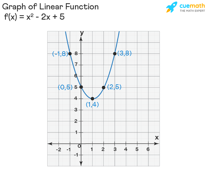
Quadratic functions produce parabolas—symmetrical U-shaped (or inverted U-shaped) curves. The standard form is y = ax² + bx + c. The sign of a determines the direction of the parabola: positive a opens upwards, negative a opens downwards. The vertex (the highest or lowest point) and the x-intercepts (roots) are key features. Parabolas are frequently encountered in physics (e.g., projectile motion) and engineering, modeling phenomena that exhibit a single turning point or symmetrical curvature. Identifying a quadratic graph involves looking for this distinct symmetrical curve, often with a clear minimum or maximum point.

Exponential and Logarithmic Functions

Exponential functions, typically in the form y = ab^x or y = ae^(kx), are characterized by rapid growth or decay. Their graphs are smooth curves that either increase very quickly or decrease very quickly, approaching an asymptote (a line that the graph gets infinitely close to but never touches). Logarithmic functions, y = log_b(x), are the inverses of exponential functions, exhibiting very slow growth for large x values. These functions are crucial in modeling population growth, radioactive decay, compound interest, and phenomena where the rate of change is proportional to the current quantity. Visually, exponential graphs show a steepening curve, while logarithmic graphs show a flattening curve, both often hugging an axis.

Polynomial Functions of Higher Degree

Polynomial functions of degree three or higher (e.g., cubic y = ax³ + bx² + cx + d, quartic, etc.) have more complex, undulating shapes. They can have multiple turning points (local maxima and minima) and inflection points. The general shape is determined by the highest power of x (the degree) and the leading coefficient. For instance, a cubic function will have up to two turning points. While more complex to fit manually, understanding their characteristic “wavy” or “S-shaped” patterns is important, as they can model more intricate relationships in data, such as economic cycles or complex engineering responses.

Trigonometric Functions (Sine, Cosine)

Trigonometric functions like y = A sin(Bx + C) + D and y = A cos(Bx + C) + D describe periodic phenomena—patterns that repeat over regular intervals. Their graphs are characteristic waves with a distinct amplitude (height), period (length of one cycle), and phase shift (horizontal displacement). They are indispensable for modeling oscillations, waves, sound, light, and seasonal patterns. Recognizing these involves identifying a clear, repeating wave pattern, determining its maximum and minimum values, and measuring the length of one complete cycle.

Manual Techniques for Function Derivation

While technology offers powerful tools, a solid understanding of manual techniques is essential for developing intuition and for scenarios where computational tools might be overkill or unavailable. These methods rely on analytical reasoning and basic algebra to extract the function’s parameters from key points on the graph.

Point-Slope and Two-Point Form (Linear)

For a linear function, if you can identify two distinct points on the line, say (x₁, y₁) and (x₂, y₂), you can derive the equation.

Calculate the slope (m): m = (y₂ - y₁) / (x₂ - x₁)
Use the point-slope form: y - y₁ = m(x - x₁)
Rearrange to slope-intercept form: y = mx + b. Substitute m and one of the points (x₁, y₁) into the point-slope form, then solve for b. This approach is precise and fundamental for any straight-line graph.

Using Key Points for Quadratic Functions

Deriving a quadratic function manually can be more involved but is achievable with key information:

Vertex Form: If the vertex (h, k) is clearly identifiable, use the form y = a(x - h)² + k. Then, choose any other point (x, y) on the parabola, substitute its coordinates, and solve for a.
Intercept Form: If the x-intercepts (r₁, 0) and (r₂, 0) are known, use the form y = a(x - r₁)(x - r₂). Again, pick another point (x, y) on the curve to solve for a.
Standard Form (System of Equations): If you can identify three non-collinear points (x₁, y₁), (x₂, y₂), (x₃, y₃) on the parabola, substitute each into y = ax² + bx + c. This will create a system of three linear equations with three unknowns (a, b, c), which can then be solved simultaneously. This method is robust but requires careful algebraic manipulation.

Identifying Asymptotes and Intercepts

For exponential, logarithmic, and rational functions, asymptotes and intercepts are crucial clues:

Horizontal Asymptotes: For exponential functions y = ab^x + c, the horizontal asymptote is y = c. This represents the value the function approaches as x tends to positive or negative infinity.
Vertical Asymptotes: For logarithmic functions y = a log_b(x - h) + k, the vertical asymptote is x = h. For rational functions y = P(x) / Q(x), vertical asymptotes occur where the denominator Q(x) is zero (and the numerator is not).
Intercepts: The y-intercept occurs where x = 0, and x-intercepts (roots) occur where y = 0. These points provide concrete coordinates to help solve for unknown parameters in your chosen function type.

Pattern Recognition and Transformation

Many complex functions can be viewed as transformations of simpler, parent functions (e.g., y = x², y = e^x, y = sin(x)).

Shifts: A vertical shift +k moves the graph up, -k moves it down. A horizontal shift (x - h) moves it right, (x + h) moves it left.
Stretches/Compressions: A coefficient a multiplying the function (a*f(x)) causes a vertical stretch/compression. A coefficient b inside the function f(bx) causes a horizontal compression/stretch.
Reflections: A negative sign (-f(x)) reflects the graph across the x-axis, and f(-x) reflects it across the y-axis.

By observing how a given graph differs from a known parent function, you can deduce the transformation parameters and, consequently, the function’s equation. This method relies heavily on visual intuition and a strong grasp of function transformations.

Leveraging Technology for Advanced Curve Fitting

While manual methods are foundational, modern technology provides powerful and efficient tools for deriving functions from graphs, especially when dealing with large datasets, noisy data, or complex function types. These tools range from simple online calculators to sophisticated programming libraries.

Online Graphing Calculators (Desmos, GeoGebra, Wolfram Alpha)

These platforms offer intuitive graphical interfaces to explore functions and data.

Desmos: Allows users to plot points and then use its built-in regression feature (e.g., y₁ ~ mx₁ + b for linear, y₁ ~ ax₁² + bx₁ + c for quadratic) to find the best-fit equation. It provides real-time adjustments and visual feedback, making it excellent for exploration and educational purposes.
GeoGebra: Combines geometry, algebra, spreadsheets, graphing, statistics, and calculus into one easy-to-use package. It has powerful curve fitting tools and can handle various types of regression.
Wolfram Alpha: Acts as a computational knowledge engine. You can input data points or describe a graph, and it can attempt to find the underlying function, often providing multiple potential models and their goodness of fit. It’s particularly useful for symbolic computation and more complex function types.

Spreadsheet Software (Microsoft Excel, Google Sheets)

Spreadsheets are ubiquitous tools for data analysis and visualization, offering robust features for curve fitting:

Scatter Plot: Create a scatter plot of your data points.
Add Trendline: Right-click on the data points and select “Add Trendline.”
Choose Function Type: Excel offers several built-in trendline types: Linear, Exponential, Logarithmic, Polynomial (up to degree 6), and Power.
Display Equation and R-squared: Crucially, check the options to “Display Equation on chart” and “Display R-squared value on chart.” The R-squared value indicates how well the trendline fits the data (closer to 1 is better).

This method is straightforward for common function types and provides immediate visual and statistical feedback on the fit.

Programming Languages and Libraries (Python with NumPy, SciPy, Matplotlib)

For advanced users, larger datasets, or custom function types, programming languages offer unparalleled flexibility and power. Python, with its rich ecosystem of libraries, is a popular choice:

NumPy (numpy.polyfit): For polynomial regression, numpy.polyfit(x_data, y_data, degree) can calculate the coefficients of a polynomial that best fits your data in a least squares sense. This is highly efficient for polynomial models.
SciPy (scipy.optimize.curve_fit): This is a more general and powerful function for non-linear least squares fitting. You define your desired function (def func(x, a, b, c): return a * np.exp(b * x) + c) and curve_fit will find the optimal parameters (a, b, c) that best fit your data. This is invaluable for exponential, logarithmic, trigonometric, and custom mathematical models.
Matplotlib: While not for fitting, Matplotlib is essential for visualizing your data, the fitted curve, and residuals, allowing for qualitative assessment of the fit.

These tools enable highly customizable and scalable solutions for function derivation, integrating seamlessly into broader data analysis workflows.

Dedicated Statistical Software (R, MATLAB)

For professionals in statistics, engineering, and scientific research, dedicated statistical software packages provide even more comprehensive capabilities:

R: A powerful open-source language and environment for statistical computing and graphics. It offers extensive packages for linear models (lm()), generalized linear models (glm()), and non-linear regression (nls()) to fit virtually any function to data. R’s strength lies in its statistical rigor and vast community support.
MATLAB: A proprietary programming platform optimized for numerical computation, visualization, and algorithm development. Its polyfit, fit, and lsqcurvefit functions provide robust tools for various types of curve fitting, alongside powerful data visualization and analysis features, particularly favored in engineering and scientific simulations.

Best Practices and Considerations

Deriving a function from a graph isn’t just about applying a formula or using a tool; it requires critical thinking and an understanding of the underlying data and potential pitfalls.

Data Quality and Outliers

The accuracy of your derived function is heavily dependent on the quality of your input data. Outliers—data points that significantly deviate from the general pattern—can heavily skew regression results, leading to an inaccurate function. It’s crucial to identify, analyze, and, if appropriate, handle outliers (e.g., removal, transformation) before fitting a function. Visual inspection of the graph is key for this initial data sanity check.

Choosing the Right Model: Overfitting vs. Underfitting

Selecting the appropriate function type is paramount.

Underfitting: Occurs when the chosen function is too simple to capture the underlying patterns in the data (e.g., using a linear function for clearly quadratic data). The model will have high bias and poor performance on both training and new data.
Overfitting: Occurs when the chosen function is too complex and fits the noise in the data rather than the true underlying relationship (e.g., using a 10th-degree polynomial for a slightly curved dataset). The model will fit the training data extremely well but perform poorly on new, unseen data due to high variance.

The goal is to find the “sweet spot”—a model complex enough to capture the signal but simple enough not to capture the noise. Occam’s Razor, which suggests choosing the simplest explanation that fits the evidence, is a good guiding principle here.

Interpreting Results: Understanding R-squared and Residuals

Once a function is derived, evaluating its goodness of fit is critical:

R-squared (Coefficient of Determination): This value, ranging from 0 to 1, indicates the proportion of the variance in the dependent variable (y) that is predictable from the independent variable (x). An R-squared closer to 1 suggests a better fit, but it doesn’t guarantee the model is correct or appropriate.
Residuals: These are the differences between the observed y values and the y values predicted by your function. Plotting residuals against x can reveal patterns (e.g., a systematic curve in the residuals) that indicate the chosen function type is inappropriate, even if the R-squared value is high. A good fit will show randomly scattered residuals around zero.

Limitations and Assumptions

Remember that every model makes assumptions. For instance, linear regression assumes a linear relationship, independent errors, and homoscedasticity (constant variance of errors). Violating these assumptions can lead to misleading results. Sometimes, a single mathematical function may not perfectly describe a real-world phenomenon across its entire domain. In such cases, piecewise functions (different functions for different ranges of x) or more advanced statistical modeling techniques might be necessary. Always consider the context of the data and the purpose of the model when interpreting your findings.

The ability to derive a function from a graph is a cornerstone skill in technical proficiency. It empowers individuals to move beyond mere observation to deep quantitative understanding. By combining a solid grasp of basic mathematical function types, effective manual derivation techniques, and the judicious application of powerful technological tools, you can accurately translate visual data into actionable mathematical models. Embrace the iterative process of fitting, evaluating, and refining your models, and you will unlock profound insights hidden within the lines and curves of your data.

aViewFromTheCave is a participant in the Amazon Services LLC Associates Program, an affiliate advertising program designed to provide a means for sites to earn advertising fees by advertising and linking to Amazon.com. Amazon, the Amazon logo, AmazonSupply, and the AmazonSupply logo are trademarks of Amazon.com, Inc. or its affiliates. As an Amazon Associate we earn affiliate commissions from qualifying purchases.