
In the vast landscape of data and digital information, understanding the relationship between visual representations and their underlying mathematical structures is a cornerstone of modern technology. Graphs are ubiquitous – from displaying stock market trends and scientific experimental results to visualizing sensor data and user engagement metrics. While a graph provides immediate visual insight, its true power often lies in the ability to distill that visual information into a concise, actionable mathematical equation. This process of extracting an equation from a graph is not merely an academic exercise; it’s a critical skill for engineers, data scientists, software developers, and researchers across countless technological domains.
An equation serves as a predictive model, a tool for interpolation and extrapolation, and a compact way to describe complex relationships. It allows us to automate calculations, integrate data into software applications, and build more sophisticated algorithms. This article delves into the methodologies and technological tools available to transform graphical data into robust mathematical equations, positioning this skill firmly within the realm of tech proficiency.
Understanding the Fundamentals: Why Equations Matter
The ability to derive an equation from a graphical representation is more than just a mathematical trick; it’s a fundamental step in translating raw data into actionable intelligence. In a world increasingly driven by data, the capacity to model real-world phenomena mathematically is a prerequisite for innovation.
The Power of Mathematical Modeling
At its core, finding an equation from a graph is about mathematical modeling. A graph presents a visual narrative of how one variable relates to another. An equation, then, becomes the precise mathematical language describing that narrative. For instance, in software engineering, performance metrics might be graphed over time. Deriving an equation allows engineers to predict future performance, identify bottlenecks, or optimize resource allocation based on a predictive model rather than relying solely on past observations. Similarly, in AI and machine learning, many algorithms implicitly or explicitly seek to find the “best-fit” equation (or function) that describes the relationship within a given dataset, often visualized as scatter plots or complex multi-dimensional graphs. This modeling capability enables simulation, prediction, and control, which are vital components of advanced technological systems.
Bridging Data Visualization and Analysis
Data visualization tools are paramount in tech for making complex datasets understandable. However, visualization is only the first step. To move from understanding to action, one often needs to analyze the underlying patterns rigorously. An equation bridges this gap. A line graph showing a steady increase in user sign-ups, for example, can be approximated by a linear equation. This equation then allows a product manager to project future growth, a marketing team to set targets, or an infrastructure team to plan server capacity. Without the equation, these decisions would be based on visual estimation, which lacks precision and the ability to be easily integrated into automated systems or further mathematical analysis. Thus, the equation elevates the perceived insights from a graph into quantifiable, verifiable, and programmable knowledge.
Identifying Key Graph Characteristics
The first step in finding an equation from a graph, whether performed manually or with technological assistance, is to thoroughly understand the graph’s visual properties. These characteristics often hint at the type of function that best describes the data.
Recognizing Common Function Types
Different patterns on a graph correspond to different families of equations. Recognizing these patterns is crucial:
-
Linear Functions: A straight line indicates a linear relationship ($y = mx + b$). This is common in simple growth models, constant rates of change, or direct proportionality.
-
Quadratic Functions: A parabola suggests a quadratic relationship ($y = ax^2 + bx + c$). These appear in projectile motion, optimization problems (finding maximum/minimum points), or the efficiency curves of certain algorithms.
-
Exponential Functions: A curve that increases or decreases at an accelerating rate (e.g., population growth, radioactive decay, compound interest) points to an exponential equation ($y = ab^x$).
-
Logarithmic Functions: A curve that initially rises quickly but then levels off (e.g., diminishing returns, Richter scale) often implies a logarithmic relationship ($y = a log(x) + b$).
-
Sinusoidal Functions: Oscillating or wave-like patterns are characteristic of trigonometric functions ($y = A sin(Bx + C) + D$), frequently seen in signal processing, periodic data (like seasonal sales or daily temperature cycles), or wave mechanics.
-
Polynomial Functions: More complex curves with multiple turning points might require higher-order polynomial equations ($y = ax^n + dots + cx + d$). These are versatile for fitting a wide range of data.
Extracting Critical Points and Features
Once a potential function type is identified, the next step is to extract specific features from the graph that will help determine the constants (coefficients) in the equation:
-
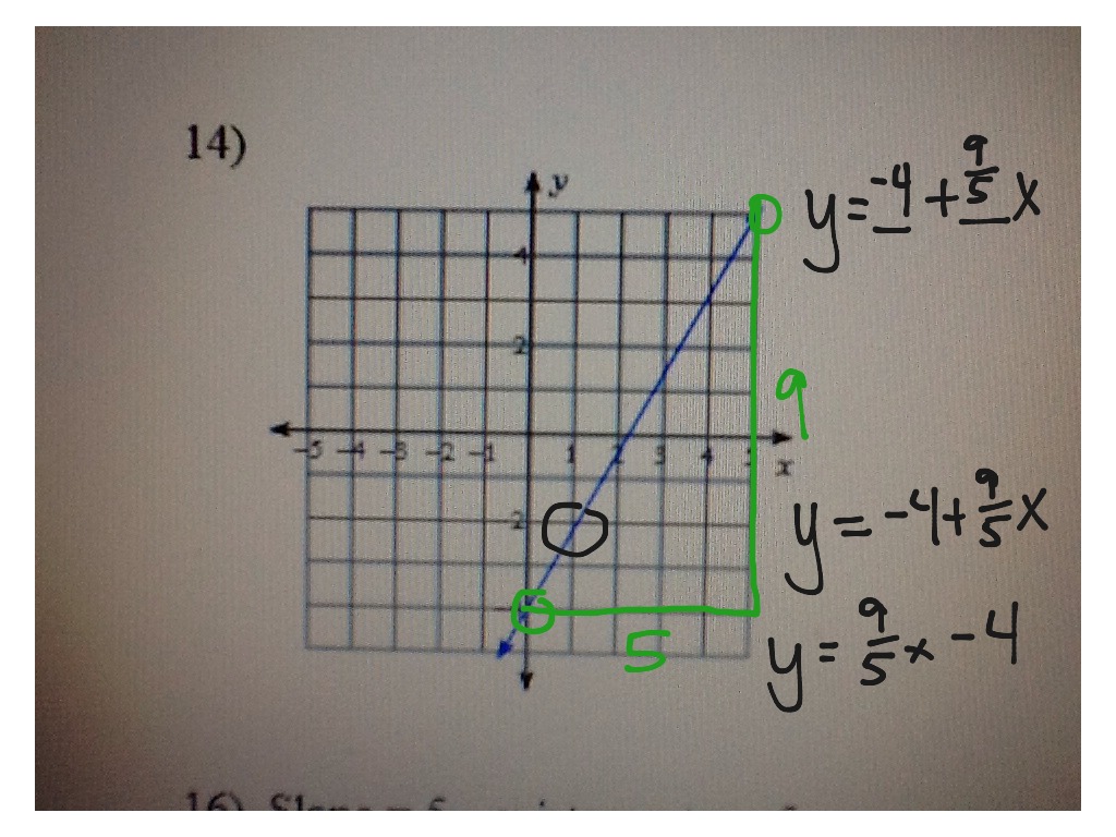
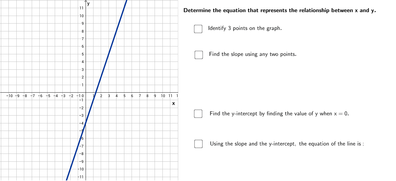
Slope and Intercepts (for linear functions): For a straight line, picking two points allows calculation of the slope ($m = frac{y2 – y1}{x2 – x1}$). The y-intercept is where the line crosses the y-axis (when $x=0$).
-
Vertex (for quadratic functions): The highest or lowest point of a parabola (the vertex $(h, k)$) is critical, as it can be directly used in the vertex form of a quadratic equation ($y = a(x-h)^2 + k$).
-
Asymptotes (for exponential, logarithmic, rational functions): Lines that the graph approaches but never touches (horizontal, vertical, or slant asymptotes) provide vital clues about the function’s behavior at extremes.
-
Period, Amplitude, Phase Shift, Vertical Shift (for sinusoidal functions): Measuring the length of one cycle, the height from the midline to the peak, and the horizontal/vertical displacement helps define the parameters of trigonometric equations.
-
Specific Points: For any function type, selecting several distinct, easily readable points from the graph provides data pairs $(x, y)$ that can be plugged into the general form of the equation to solve for unknown coefficients. The more points used, especially when spread across the graph, the more robust the derived equation will be.
Practical Approaches with Tech Tools
While the conceptual understanding of graph characteristics is vital, modern technology offers powerful tools to expedite and enhance the process of finding an equation.
Manual Techniques and Estimation
Even with advanced software, a foundational understanding of manual estimation is valuable. For simpler graphs, one can visually estimate slopes, intercepts, or vertices. For example, sketching a “best-fit” line through a scatter plot and then using two points on that line to calculate its equation is a quick, rough manual method. This approach, while less precise, builds intuition and can serve as a sanity check for results obtained from more sophisticated tools. It’s especially useful for quick analyses or when computational tools aren’t immediately available.
Leveraging Graphing Calculators and Software
The true power for deriving equations from graphs often lies in dedicated software.
-
Graphing Calculators (e.g., TI-84, Casio fx-CG50): These devices have built-in “regression” features. Users input a set of data points (taken from the graph), specify the type of regression (linear, quadratic, exponential, etc.), and the calculator computes the best-fit equation and its coefficients.
-
Online Graphing Tools (e.g., Desmos, GeoGebra): These platforms are incredibly intuitive. You can often plot points directly, or even sketch a curve, and then use their built-in regression features by entering the data or a general equation with sliders for parameters. They provide instant visual feedback on how well the derived equation fits the original graph.
-
Spreadsheet Software (e.g., Microsoft Excel, Google Sheets): Excel’s charting tools allow users to plot data and then add a “Trendline.” For this trendline, you can select various types (linear, exponential, polynomial, logarithmic) and choose to “Display Equation on chart.” Excel will automatically calculate and show the equation that best fits the plotted data points. This is an accessible and widely used method in business and casual data analysis.
Programming for Curve Fitting
For more complex scenarios, larger datasets, or automated processes, programming languages offer the most flexibility and power.
-
Python: With libraries like
NumPyandSciPy, Python is a powerhouse for curve fitting. Thenumpy.polyfit()function can find the coefficients of a polynomial that best fits a set of data points. For non-polynomial functions,scipy.optimize.curve_fit()is a more general tool, allowing users to define their own function model and then fitting it to data using non-linear least squares.MatplotliborSeaborncan then be used to visualize the original data and the fitted curve. -
MATLAB: This proprietary language is specifically designed for numerical computation. Its
polyfitfunction works similarly to NumPy’s, and thefitfunction (part of the Curve Fitting Toolbox) provides an interactive environment and robust algorithms for fitting various function types to data, including custom equations. -
R: Statistical programming languages like R also excel at this. Functions like
lm()for linear models or various packages for non-linear regression allow sophisticated curve fitting based on data points extracted from graphs.
These programmatic approaches are fundamental in data science, machine learning model development, and scientific computing, where precise control over the fitting process and the ability to handle massive datasets are critical.
Advanced Techniques and Considerations
Beyond basic curve fitting, several advanced techniques and considerations enhance the accuracy and utility of equations derived from graphs.
Polynomial Regression and Interpolation
When simple linear, exponential, or quadratic models don’t adequately capture the complexity of a graph, polynomial regression offers greater flexibility. By increasing the degree of the polynomial, one can fit increasingly intricate curves. However, care must be taken to avoid overfitting, where a high-degree polynomial fits the specific data points too closely but fails to generalize well to new, unseen data. Interpolation (finding values between known data points) is also a key application, often used to fill gaps in sensor data or generate smoother animations in graphics.
Dealing with Noisy Data and Model Validation
Real-world data, especially from sensors or experiments, is often “noisy” – containing random fluctuations or errors. Simply fitting an equation to noisy data without consideration can lead to a misleading model. Techniques like smoothing (e.g., moving averages) or robust regression methods can help. Crucially, after deriving an equation, it’s essential to validate its accuracy. This involves:
-
Residual Analysis: Examining the differences between the actual data points and the values predicted by the equation. A good fit should show small, randomly distributed residuals.
-
R-squared Value: A statistical measure (commonly used in regression) indicating the proportion of the variance in the dependent variable that is predictable from the independent variable(s). An R-squared closer to 1 (or 100%) generally indicates a better fit.
-
Cross-Validation: Splitting the data into training and testing sets. The equation is derived from the training set, and its performance is evaluated on the unseen test set to ensure generalizability.
The Role of AI and Machine Learning in Automated Curve Fitting
The future of deriving equations from graphs increasingly involves artificial intelligence and machine learning. Deep learning models, particularly neural networks, can learn complex non-linear relationships within data without explicit predefined function types. For example, a neural network could be trained on image data of graphs and learn to directly output the parameters of the best-fit equation, or even generate the equation itself. Computer vision techniques can be used to automatically extract data points from scanned or image-based graphs, feeding them into automated regression algorithms. This automation significantly speeds up the analysis of large volumes of visual data, moving from manual data extraction to fully automated pattern recognition and equation generation.

Conclusion
The ability to find an equation from a graph is a foundational skill in the tech world, bridging the gap between visual data representation and powerful mathematical modeling. From the simplest linear trends to complex non-linear relationships, extracting an equation allows for prediction, automation, and deeper analytical insight. Whether utilizing intuitive online graphing tools, robust spreadsheet functions, or advanced programmatic libraries in Python or MATLAB, the methodologies discussed here empower professionals to transform static graphs into dynamic, actionable mathematical models. As technology continues to advance, incorporating AI and machine learning, this process will become even more sophisticated and automated, further solidifying its critical role in data science, engineering, and software development. Mastering this conversion from visual to mathematical is not just about understanding data; it’s about leveraging that understanding to build the intelligent systems of tomorrow.
aViewFromTheCave is a participant in the Amazon Services LLC Associates Program, an affiliate advertising program designed to provide a means for sites to earn advertising fees by advertising and linking to Amazon.com. Amazon, the Amazon logo, AmazonSupply, and the AmazonSupply logo are trademarks of Amazon.com, Inc. or its affiliates. As an Amazon Associate we earn affiliate commissions from qualifying purchases.