
The transition toward a decentralized, renewable energy grid is fundamentally a data-driven evolution. For engineers, installers, and technology enthusiasts, the ability to accurately predict the performance of a solar photovoltaic (PV) system is not merely a convenience—it is a technical necessity. Estimating the annual energy production (AEP) of a solar array involves more than a cursory glance at weather patterns; it requires a deep dive into irradiance physics, hardware efficiency ratings, and digital simulation modeling.
To achieve a high-fidelity output, one must understand the interplay between environmental variables and the technological limitations of the hardware. This guide provides a technical roadmap for calculating annual energy production, moving from raw atmospheric data to the final kilowatt-hour (kWh) output.
The Core Variables of Solar Irradiance and Photovoltaic Efficiency
Before any hardware is mounted, the primary input variable—the sun—must be quantified. In the tech-heavy world of PV modeling, we do not simply count sunny days. Instead, we look at solar irradiance, which is the power per unit area received from the Sun in the form of electromagnetic radiation.
Understanding Peak Sun Hours (PSH)
The most common metric used in technical calculations is “Peak Sun Hours.” This is not a measurement of how many hours the sun is visible, but rather a normalized figure where one PSH equals 1,000 watts of solar energy per square meter (W/m²) for one hour. For example, if a location receives 400 W/m² for five hours, that equates to 2.0 Peak Sun Hours. Identifying the PSH for a specific geographic coordinate is the baseline for any annual production algorithm.
The Role of Global Horizontal Irradiance (GHI)
Technicians utilize Global Horizontal Irradiance (GHI) as the total amount of shortwave radiation received from above by a surface horizontal to the ground. GHI is the sum of Direct Normal Irradiance (DNI) and Diffuse Horizontal Irradiance (DHI). In advanced software modeling, DNI is particularly critical for tracking systems, while DHI becomes essential for bifacial modules that capture light reflected from the ground or scattered by the atmosphere. Modern PV designers use satellite-derived datasets, such as those from NASA’s POWER API or the National Solar Radiation Database (NSRDB), to feed these variables into their calculations.
Accounting for System Derate Factors and Losses
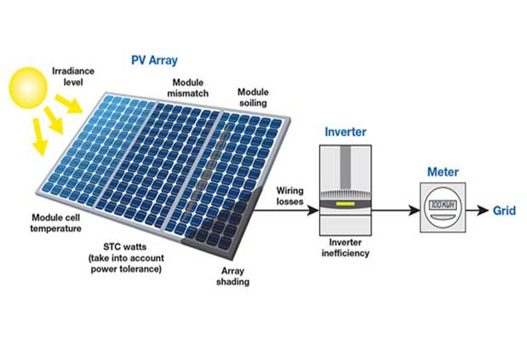
No solar technology operates at 100% efficiency in a vacuum. The difference between a panel’s “Nameplate Capacity” (the theoretical max output under Standard Test Conditions) and its actual field performance is defined by “derate factors.” These represent the inevitable losses inherent in electrical and mechanical systems.
Inverter Efficiency and Clipping
The inverter is the “brain” of the PV system, converting Direct Current (DC) from the panels into Alternating Current (AC) for the grid. Technical specifications for modern string inverters or microinverters typically show efficiencies between 96% and 99%. However, we must also account for “clipping” (inverter saturation). This occurs when the DC input exceeds the inverter’s maximum AC output capacity. While this might seem like a loss, tech-optimized systems are often designed with a DC-to-AC ratio of 1.2 to 1.4 to ensure the inverter operates at peak efficiency for a longer duration of the day.
Temperature Coefficients and Thermal Degradation
A common misconception in solar technology is that more heat equals more power. In reality, photovoltaic cells are semi-conductors that become less efficient as they get hotter. Each panel has a “temperature coefficient” (usually expressed as a percentage per degree Celsius, such as -0.35%/°C). When calculating annual production, one must factor in the ambient temperature of the site. If the module temperature rises to 65°C on a summer day, the actual power output can drop significantly compared to its performance at the 25°C Standard Test Condition (STC).
Soiling, Shading, and Wiring Losses
Digital modeling must also account for the physical environment.
- Soiling: Dust, snow, and bird droppings can create a film that reduces light transmittance, typically causing a 2% to 5% annual loss.
- Shading: Even a small amount of shade on a single cell can disproportionately reduce the output of an entire string due to the physics of serial electrical connections (though modern bypass diodes and DC optimizers mitigate this).
- Wiring (Ohmic Losses): Energy is lost as heat when electrons move through copper or aluminum conductors. Engineers typically aim for a voltage drop of less than 3% in the system design.
The Mathematical Framework for Annual Yield

Once the irradiance data and loss factors are identified, we can apply the core mathematical formula used by system designers to estimate the total energy delivered to the grid.
The Basic Calculation Formula
The fundamental equation for estimating annual energy production (E) is:
E = A × r × H × PR
Where:
- E = Energy (kWh)
- A = Total solar panel area (m²)
- r = Solar panel yield or efficiency (%)
- H = Annual average solar radiation on tilted panels (shadings not included)
- PR = Performance Ratio (the “catch-all” coefficient for losses)
The Performance Ratio (PR) is a crucial metric in the solar tech industry. It represents the relationship between the actual and theoretical energy outputs. A high-spec, well-maintained system usually boasts a PR between 0.75 and 0.85.
Factoring in Panel Orientation and Tilt Angle
The angle of incidence is a critical technical variable. In the northern hemisphere, panels are generally oriented toward true south. The tilt angle is optimized based on the latitude of the installation to maximize the “H” value in the formula above. Fixed-tilt systems are often set at an angle equal to the local latitude. However, advanced installations may use “Single-Axis Trackers,” which use automated actuators and software algorithms to follow the sun’s arc, increasing annual energy yield by 15% to 25% compared to static mounts.
Leveraging Digital Tools and Simulation Software
Manual calculations are excellent for preliminary estimates, but the complexity of modern solar arrays requires sophisticated software to account for hourly weather variations and complex 3D shading environments.
Professional Modeling with PVSyst and Helioscope
In the professional engineering niche, PVSyst is considered the gold standard. It allows for “Monte Carlo” simulations that account for nearly every technical variable, including spectral correction and LID (Light Induced Degradation). Helioscope, conversely, integrates CAD-like features with Google Maps data to provide rapid 3D overlays and wiring diagrams, automatically calculating the annual production based on the specific geometry of the roof or ground site. These tools use “Typical Meteorological Year” (TMY3) data—a dataset that represents the median weather conditions for a specific location over a 30-year period.
API Integration for Real-Time Monitoring and Forecasting
Calculating production is no longer a “one and done” event. The modern “Energy-Tech” ecosystem utilizes IoT (Internet of Things) sensors and cloud-based APIs to compare predicted yield with actual performance in real-time. If a system’s production falls below the modeled 1300 kWh/kWp (kilowatt-hours per kilowatt-peak), the software can trigger an automated alert, identifying whether the delta is caused by a hardware failure, an inverter fault, or unexpected atmospheric conditions.
Furthermore, machine learning algorithms are now being integrated into production calculations to predict “cloud transients.” By analyzing historical weather data and real-time satellite imagery, these tools can forecast the next 15 to 60 minutes of production, allowing grid operators to balance the load more effectively.
Conclusion: The Precision of the Photovoltaic Future
Calculating the annual energy production of solar panels is an exercise in technical precision. By moving beyond simple estimates and embracing the complexities of solar irradiance, thermal physics, and system derate factors, we can build a more reliable and transparent renewable energy infrastructure.
As solar cell technology advances—moving from traditional Monocrystalline Silicon to high-efficiency N-Type TopCon and Perovskite Tandem cells—the formulas and software models we use must also evolve. The goal remains constant: to transform the raw, chaotic energy of the sun into a predictable, digital stream of electrons that can be calculated, monitored, and optimized with mathematical certainty. Whether you are using a basic formula or a complex digital twin simulation, understanding the “how” behind the numbers is the key to mastering solar technology.
aViewFromTheCave is a participant in the Amazon Services LLC Associates Program, an affiliate advertising program designed to provide a means for sites to earn advertising fees by advertising and linking to Amazon.com. Amazon, the Amazon logo, AmazonSupply, and the AmazonSupply logo are trademarks of Amazon.com, Inc. or its affiliates. As an Amazon Associate we earn affiliate commissions from qualifying purchases.