How Do I Graph y = 3? A Comprehensive Tech-Driven Tutorial

Graphing mathematical equations is a fundamental skill across various fields, from science and engineering to economics and data analysis. While the simple equation “y = 3” might seem straightforward, understanding its graphical representation is a cornerstone for comprehending more complex functions and data visualizations. In an increasingly digital world, technology has transformed the way we approach graphing, making it more accessible, interactive, and powerful than ever before. This tutorial will not only guide you through the process of graphing y = 3 but will also explore the myriad technological tools that simplify and enhance this essential task.

Understanding the Fundamentals of y = 3

Before diving into the digital realm, a solid grasp of what y = 3 signifies in a mathematical context is crucial. This foundational knowledge empowers you to interpret graphs accurately, whether they’re drawn by hand or generated by a sophisticated algorithm.

Decoding the Equation: What Does y = 3 Mean?

The equation y = 3 is an example of a constant function. In a two-dimensional Cartesian coordinate system, any point is defined by its (x, y) coordinates. The equation y = 3 dictates that for any value of x, the corresponding y-value must always be 3.

Consider these points:

If x = -5, y must be 3. So, the point is (-5, 3).
If x = 0, y must be 3. So, the point is (0, 3).
If x = 10, y must be 3. So, the point is (10, 3).

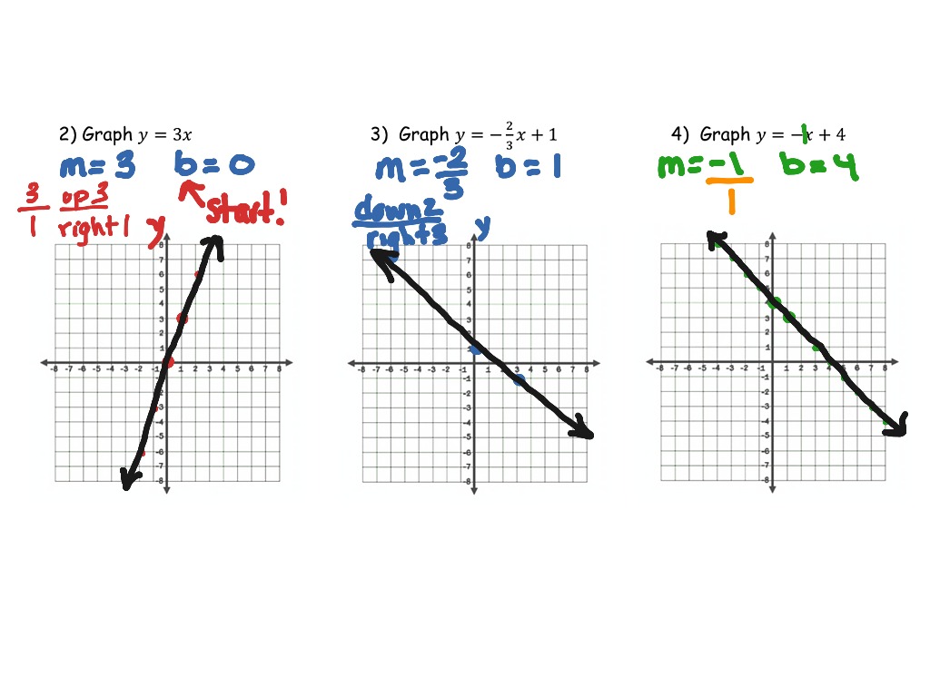
When you plot all such points where y consistently equals 3, regardless of x, they form a straight, horizontal line. This line is parallel to the x-axis and passes through the point where the y-coordinate is 3 on the y-axis. It extends infinitely in both the positive and negative x-directions. This concept is simple yet profoundly important, as it provides the basis for understanding more intricate linear and non-linear functions.

The Cartesian Coordinate System Refresher

To graph y = 3, whether manually or using software, you need to understand the Cartesian coordinate system, also known as the rectangular coordinate system.

X-axis: This is the horizontal line, representing the independent variable. Values increase to the right of the origin (0,0) and decrease to the left.
Y-axis: This is the vertical line, representing the dependent variable. Values increase above the origin and decrease below it.
Origin (0,0): The point where the x-axis and y-axis intersect. It serves as the reference point for all other coordinates.
Quadrants: The x and y axes divide the plane into four quadrants, numbered counter-clockwise starting from the top-right.

Every point in this system can be uniquely identified by an ordered pair (x, y). For y = 3, we are looking for all points where the vertical position is fixed at 3 units above the x-axis.

Manual Graphing: The Foundational Skill

Even with the abundance of digital tools, understanding how to manually graph is essential. It builds intuition and problem-solving skills, making you a more adept user of technology rather than just a passive observer.

Step-by-Step Manual Plotting of y = 3

Draw the Axes: On a piece of graph paper, draw a horizontal line (x-axis) and a vertical line (y-axis) intersecting at a central point (the origin).
Label and Scale the Axes: Mark units along both axes. For instance, label 1, 2, 3… to the right and left on the x-axis, and up and down on the y-axis. Ensure consistent scaling for clarity.
Identify Key Points: Since y is always 3, pick a few simple x-values to visualize. For example:
- (0, 3) – The point where the line crosses the y-axis.
- (2, 3)
- (-4, 3)
Plot the Points: Locate these points on your graph paper and mark them with a small dot.
Draw the Line: Using a ruler, draw a straight line that passes through all the plotted points. This line should be perfectly horizontal. Extend the line beyond your plotted points and add arrows at both ends to indicate that it continues indefinitely.
Label the Line: Write “y = 3” next to the line to clearly identify the equation it represents.

Common Pitfalls in Manual Graphing

While simple, manual graphing can still present challenges:

Confusing Axes: A frequent mistake is drawing a vertical line at x=3 instead of a horizontal line at y=3. Remember, “y=constant” means a horizontal line, and “x=constant” means a vertical line.
Incorrect Scaling: Inconsistent or poorly chosen scales can distort the visual representation, especially for more complex equations.
Lack of Precision: Freehand lines or poorly marked points can lead to inaccurate graphs. Always use a ruler and sharp pencil.
Not Extending the Line: A line representing an equation extends infinitely; not drawing arrows or extending the line suggests a segment rather than a continuous function.

Leveraging Technology for Graphing y = 3

The true power of modern technology shines in its ability to graph equations with speed, precision, and interactivity. From simple online tools to advanced programming environments, numerous options exist to visualize y = 3 and far more complex functions.

Online Graphing Calculators: Desmos and GeoGebra

Online graphing calculators are perhaps the most accessible and user-friendly tools for visualizing mathematical functions. They are free, web-based, and offer immediate results.

Desmos Graphing Calculator

Desmos is renowned for its intuitive interface and dynamic capabilities.

Access Desmos: Open your web browser and navigate to desmos.com/calculator.
Input the Equation: In the left-hand panel, you’ll see an input box. Simply type y = 3.
Instant Graph: As soon as you type, Desmos will instantly draw the horizontal line at y=3 on the coordinate plane.
Explore Features:
- Zoom/Pan: Use your mouse wheel or trackpad to zoom in/out and click-and-drag to pan the graph.
- Add More Equations: You can add x = 2 or y = x to see how y=3 interacts with other lines.
- Tables: Desmos can generate a table of values if needed, although for y=3 it’s trivially all 3s.
- Labels: You can add labels or notes to your graph for presentation.

GeoGebra Classic

GeoGebra is another powerful and versatile tool, offering graphing, geometry, 3D, and spreadsheet functionalities.

Access GeoGebra: Go to geogebra.org/classic.
Input the Equation: At the bottom, there’s an “Input” bar. Type y = 3 and press Enter.
Automatic Plotting: GeoGebra will display the graph of y=3.
Interactive Elements:
- Move Graphics View: Use the “Move Graphics View” tool (hand icon) to pan.
- Zoom In/Out: Use the scroll wheel or the zoom buttons.
- Points: You can explicitly add points like (0, 3) using the input bar to see them on the line.

Both Desmos and GeoGebra are excellent for students, educators, and anyone needing quick, accurate, and interactive graphing.

Dedicated Graphing Software and Programming Environments

For more advanced needs, professional-grade software and programming libraries offer greater control, customization, and analytical capabilities.

Wolfram Alpha

While not a dedicated graphing calculator in the traditional sense, Wolfram Alpha is a computational knowledge engine that can interpret and graph mathematical expressions.

Visit Wolfram Alpha: Go to wolframalpha.com.
Input Query: Type graph y = 3 into the search bar and press Enter.
Detailed Output: Wolfram Alpha will not only display the graph but also provide properties of the line (e.g., slope, intercept, alternate forms), making it a comprehensive learning tool.

MATLAB/Octave

For engineers, scientists, and advanced students, MATLAB (or its open-source alternative, Octave) is a powerful numerical computing environment.

Define X-values: In the command window, you’d first define a range for x:

x = -10:1:10; (This creates x values from -10 to 10 with steps of 1)
Define Y-values: Since y is constant:

y = 3 * ones(size(x)); (This creates a vector of 3s with the same size as x)
Plot:

plot(x, y);

grid on; (Adds a grid for clarity)

xlabel('x-axis'); ylabel('y-axis'); title('Graph of y = 3'); (Adds labels)

This approach provides full control over plot aesthetics and allows for integration into larger scripts for data analysis or simulations.

Python with Matplotlib

Python, with its matplotlib library, is a popular choice for data visualization and scientific computing due to its flexibility and open-source nature.

Import Matplotlib:

import matplotlib.pyplot as plt

import numpy as np
Define X and Y:

x = np.linspace(-10, 10, 100) (Generates 100 evenly spaced points between -10 and 10)

y = np.full_like(x, 3) (Creates an array of 3s, matching the size of x)
Plot:

plt.plot(x, y)

plt.xlabel('x-axis')

plt.ylabel('y-axis')

plt.title('Graph of y = 3')

plt.grid(True)

plt.axhline(0, color='black', linewidth=0.5) (Adds x-axis line)

plt.axvline(0, color='black', linewidth=0.5) (Adds y-axis line)

plt.show()

Python offers unparalleled customization for plots, suitable for research, professional reports, and complex data visualizations.

Smartphone Apps for On-the-Go Graphing

For convenience and portability, numerous smartphone apps can graph equations. Apps like Photomath, Microsoft Math Solver, and dedicated graphing calculator apps (e.g., Graphing Calculator by Mathlab) allow you to input equations and immediately see their graphical representation. Some even offer augmented reality features, letting you graph equations by scanning them from a textbook. These tools are perfect for quick checks, homework, or understanding concepts while away from a computer.

Beyond Basic Graphing: Enhancing Understanding with Tech

Technology doesn’t just graph; it helps deepen understanding by allowing dynamic exploration and visualization of mathematical relationships.

Visualizing Transformations

With digital tools, it’s easy to see how y=3 relates to other functions.

Shifts: Graph y = 3 alongside y = x + 3 or y = 3x. Notice how y=3 acts as a baseline, showing a y-intercept or a horizontal translation.
Varying Constants: Many tools allow you to use sliders for constants. Imagine graphing y = k and using a slider for k. You’d see the horizontal line move up and down in real-time as k changes, providing a powerful visual demonstration of the parameter’s effect.

Intersections and Systems of Equations

Graphing y=3 with another equation helps visualize solutions to systems of equations. For example, if you graph y = 3 and x + y = 5, Desmos or GeoGebra will automatically show the intersection point (2, 3), representing the solution where both equations are true. This interactive visualization is far more intuitive than purely algebraic methods for many learners.

Parameterization and Dynamic Graphing

Advanced graphing tools can handle parameterized equations or dynamic variables. While y=3 is fixed, understanding that it’s a specific instance of y=k (where k is a parameter) can be explored dynamically. Some tools allow for animation, which, while not directly applicable to a static line like y=3, demonstrates how graphical representations evolve under changing conditions, preparing users for more complex scenarios in physics or engineering.

Choosing the Right Tool for Your Graphing Needs

The best tool depends on your specific requirements, skill level, and the complexity of the task.

Simplicity vs. Complexity

For quick checks, basic understanding, or homework: Online calculators like Desmos or GeoGebra, or smartphone apps, are ideal. They are user-friendly, fast, and free.
For detailed analysis, custom plots, or integration into larger projects: MATLAB, Octave, or Python with Matplotlib offer the flexibility and power needed. These require a steeper learning curve but provide unparalleled control.
For academic research or in-depth problem-solving with additional computational context: Wolfram Alpha provides not just graphs but also properties and related mathematical information.

Learning Curve and Accessibility

Online calculators and smartphone apps generally have the lowest learning curve, often requiring just a few minutes to grasp the basics.
Programming environments like Python or MATLAB require familiarity with coding concepts, making their learning curve significantly higher, but the investment pays off in versatility.

Integration with Other Tools

Consider if your graphing needs are isolated or part of a larger workflow. Python and MATLAB excel in environments where graphing is one component of a broader data analysis, simulation, or report generation process, allowing for seamless integration.

Conclusion

Graphing y = 3 is a foundational exercise in mathematics that beautifully illustrates the relationship between an equation and its visual representation in a coordinate plane. While manual plotting builds essential intuition, technology dramatically streamlines and enhances the process. From accessible online calculators like Desmos and GeoGebra to powerful programming environments like Python and MATLAB, a vast array of tools exists to help you visualize mathematical concepts with precision and interactivity.

By embracing these technological advancements, you can move beyond simply plotting points to truly understanding the dynamics of functions, interpreting complex data, and solving intricate problems. Whether you’re a student, educator, or professional, mastering the art of tech-driven graphing is an invaluable skill that unlocks deeper insights into the world of mathematics and beyond. So, go forth and explore – the horizontal line at y=3 is just the beginning of your graphing journey!

aViewFromTheCave is a participant in the Amazon Services LLC Associates Program, an affiliate advertising program designed to provide a means for sites to earn advertising fees by advertising and linking to Amazon.com. Amazon, the Amazon logo, AmazonSupply, and the AmazonSupply logo are trademarks of Amazon.com, Inc. or its affiliates. As an Amazon Associate we earn affiliate commissions from qualifying purchases.