
In the intricate world of data science, machine learning, and statistical modeling, precision and reliability are paramount. As technology increasingly relies on sophisticated algorithms and vast datasets, understanding the underlying statistical assumptions and potential pitfalls becomes critical. One such fundamental concept, often overlooked but deeply impactful, is heteroscedasticity. At its core, heteroscedasticity describes a condition in statistical models, particularly regression analysis, where the variability of the errors, or residuals, is not constant across all levels of the independent variables. This phenomenon can significantly undermine the validity and efficiency of models, making it a crucial topic for any tech professional involved in data analysis, algorithm development, or AI tool deployment.
Understanding the Variability in Data Models
To grasp heteroscedasticity, it’s essential to first understand its counterpart: homoscedasticity. In an ideal regression model, we assume that the error term, representing the unexplained variance after accounting for the independent variables, is constant across all observations. This state, where the spread of the residuals remains uniform as the predicted value changes, is known as homoscedasticity. Visually, if you plot the residuals against the predicted values, the points would form a roughly horizontal band, showing no discernable pattern in their dispersion.
Heteroscedasticity, however, signals a deviation from this ideal. It means the variance of the error term changes depending on the value of the independent variable. For instance, the errors might be small when the independent variable is low and become much larger as the independent variable increases, or vice-versa. Imagine predicting house prices based on square footage. It’s plausible that prediction errors for small, inexpensive homes are relatively minor, but for large, luxury properties, the range of possible errors (both under- and over-estimations) could be much wider due to unique features, amenities, and market nuances that are not fully captured by square footage alone. This increasing spread of errors as the independent variable increases is a classic example of heteroscedasticity.
The error term itself is a critical component of any statistical model. It represents all the factors influencing the dependent variable that are not included in the model’s independent variables. When the variance of these errors isn’t constant, it implies that the model’s ability to explain the variance of the dependent variable differs across different ranges of the independent variables. This non-constant error variance violates one of the core assumptions of Ordinary Least Squares (OLS) regression, a cornerstone algorithm in many data analysis and machine learning applications.
Why Heteroscedasticity Poses a Challenge in Tech and AI
The presence of heteroscedasticity can have severe ramifications for the reliability and interpretation of statistical models, particularly those deployed in AI systems and data-driven software. For tech professionals, understanding these implications is key to building robust and trustworthy solutions.
Firstly, heteroscedasticity does not bias the coefficient estimates themselves. That is, the estimated relationships between the independent and dependent variables will still be correct on average. However, it does make these estimates less efficient, meaning they are not the best possible estimates in terms of having the lowest variance. More critically, heteroscedasticity leads to biased and inconsistent estimates of the standard errors of the regression coefficients. Standard errors are fundamental for hypothesis testing and constructing confidence intervals, which are used to determine the statistical significance of predictors and the precision of the estimates.
When standard errors are underestimated (a common scenario with heteroscedasticity), coefficients might appear statistically significant when they are not, leading to incorrect inferences about the importance of various features in an AI model. Conversely, if standard errors are overestimated, truly significant features might be overlooked. This has profound implications for feature selection in machine learning, model optimization, and the overall interpretability of an AI system. For example, in a financial forecasting model, incorrectly attributing significance to a weak predictor could lead to poor investment decisions. In a healthcare diagnostic tool, misinterpreting the importance of a biomarker could compromise patient care.
Furthermore, heteroscedasticity can impact the predictive accuracy and generalization ability of models. While the OLS estimator remains unbiased, its inefficiency means that the prediction intervals generated by the model will be inaccurate. This can lead to overconfidence in predictions for some data points and underconfidence for others. In AI applications where precise uncertainty quantification is vital – such as autonomous driving systems needing to accurately gauge the reliability of their environmental predictions – the effects of heteroscedasticity can be detrimental to performance and safety. Software engineers building recommendation engines, anomaly detection systems, or predictive maintenance tools must contend with these issues to ensure their applications provide accurate and dependable outputs.
Identifying Heteroscedasticity: Tools and Techniques for Data Professionals

Detecting heteroscedasticity is the first step toward mitigating its adverse effects. Fortunately, data scientists and software developers have access to several effective tools and techniques for identification.
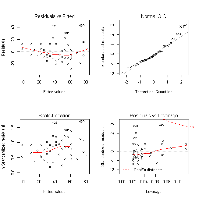
One of the most intuitive and widely used methods is visual inspection of residual plots. After fitting a regression model, plotting the residuals (the differences between observed and predicted values) against the predicted values or against each independent variable can reveal patterns indicative of heteroscedasticity. A classic sign is a “fan” or “cone” shape, where the spread of residuals widens or narrows as the predicted values increase. Other patterns, like a “diamond” shape, also suggest non-constant variance. Most statistical software packages and data analysis libraries (e.g., Python’s matplotlib and seaborn with statsmodels) provide easy ways to generate these diagnostic plots.
While visual inspection is helpful, it is subjective. For more rigorous assessment, statistical tests are employed. Two common tests include the Breusch-Pagan test and the White test.
The Breusch-Pagan test assesses whether the squared residuals are linearly related to the independent variables. If a significant relationship is found, it suggests the presence of heteroscedasticity.
The White test is a more general test that doesn’t assume a specific form of heteroscedasticity. It involves regressing the squared residuals on the original independent variables, their squared terms, and their cross-products. A significant result from the White test indicates heteroscedasticity.
Both tests yield a p-value, and if this p-value is below a chosen significance level (e.g., 0.05), the null hypothesis of homoscedasticity is rejected in favor of heteroscedasticity. Many advanced analytics platforms and programming libraries include built-in functions for performing these tests, making automated detection a routine part of model validation pipelines.
Strategies for Addressing Heteroscedasticity in Practical Applications
Once heteroscedasticity is detected, various strategies can be employed to correct or mitigate its impact, ensuring the robustness and accuracy of models in tech applications. The choice of method often depends on the nature of the data and the specific goals of the analysis.
One common approach involves data transformations. By applying mathematical transformations to the dependent variable, or sometimes to the independent variables, it’s often possible to stabilize the variance of the error term. Common transformations include:
- Logarithmic transformation: Taking the natural logarithm of the dependent variable is effective when the variance increases proportionally with the mean of the dependent variable (e.g., incomes, sales figures).
- Square root transformation: Useful when the variance is related to the count data or when the dependent variable exhibits a Poisson distribution.
- Reciprocal transformation: Can be applied when the variance is inversely proportional to the mean.
The challenge with transformations is that they change the interpretation of the coefficients. A coefficient from a log-transformed model, for example, represents a percentage change rather than a direct unit change.
Another powerful technique involves using robust standard errors, also known as heteroscedasticity-consistent standard errors (HCSE). The most widely used approach is White’s heteroscedasticity-consistent estimator. Instead of transforming the data or trying to model the heteroscedasticity, robust standard errors adjust the calculation of the standard errors to account for the non-constant variance. This means the coefficient estimates themselves remain the same, but their associated standard errors (and thus p-values and confidence intervals) are corrected, leading to more reliable hypothesis tests and inferences. Many statistical software packages and machine learning libraries (e.g., statsmodels in Python) offer options to compute robust standard errors for OLS models, making this a practical and often preferred solution in many tech contexts.
A more advanced method is Weighted Least Squares (WLS). If the form of heteroscedasticity is known or can be estimated (i.e., we can estimate how the variance of the errors changes), WLS can be applied. WLS assigns different weights to different observations during the regression process, giving less weight to observations with larger error variances and more weight to observations with smaller error variances. This effectively “downweights” the noisy observations, leading to more efficient and reliable coefficient estimates. Implementing WLS requires careful estimation of the weights, which can sometimes be complex, but it can yield superior results when the weighting scheme is accurate.
Finally, exploring alternative modeling approaches can also be a viable solution. While OLS assumes homoscedasticity, other models are inherently more robust to or explicitly designed to handle non-constant variance. For instance:
- Generalized Linear Models (GLMs): These models, such as Poisson regression for count data or logistic regression for binary outcomes, often have error distributions that naturally accommodate varying variances.
- Tree-based models (e.g., Random Forests, Gradient Boosting Machines): These non-parametric models do not rely on the same strict statistical assumptions as linear regression and are generally more robust to heteroscedasticity. They are widely used in modern AI and machine learning for their predictive power and flexibility.
The Broader Context: Data Quality and Model Robustness
In the rapidly evolving landscape of technology and artificial intelligence, the ability to build models that are not only performant but also reliable and interpretable is paramount. Understanding and addressing heteroscedasticity is not merely a statistical formality; it’s a critical component of ensuring data quality and model robustness.
By conscientiously identifying and handling heteroscedasticity, tech professionals can:
- Enhance Model Trustworthiness: Ensure that the statistical inferences drawn from models are accurate, leading to more dependable insights and decisions.
- Improve Predictive Confidence: Generate more accurate prediction intervals, providing a realistic assessment of the uncertainty associated with model forecasts, crucial for risk assessment in AI applications.
- Optimize Feature Selection: Avoid misidentifying significant features, leading to more parsimonious and effective models.
- Foster Reproducibility: Create models whose findings are more likely to hold up under scrutiny and across different datasets, a cornerstone of scientific computing and AI research.
As AI tools and data-driven software become increasingly integrated into critical infrastructures and decision-making processes, the statistical rigor underpinning these technologies cannot be overstated. Heteroscedasticity, while a seemingly technical concept, underscores the broader principle that a deep understanding of data properties and model assumptions is indispensable for developing reliable, efficient, and ethical technological solutions.
aViewFromTheCave is a participant in the Amazon Services LLC Associates Program, an affiliate advertising program designed to provide a means for sites to earn advertising fees by advertising and linking to Amazon.com. Amazon, the Amazon logo, AmazonSupply, and the AmazonSupply logo are trademarks of Amazon.com, Inc. or its affiliates. As an Amazon Associate we earn affiliate commissions from qualifying purchases.