Mastering Your Graphing Calculator: A Comprehensive Tutorial

In an era increasingly dominated by sophisticated software and AI tools, the humble graphing calculator might seem like a relic. Yet, for students, engineers, and scientists across various disciplines, this powerful handheld device remains an indispensable tool. Far more than just a glorified arithmetic machine, a graphing calculator is a dynamic educational companion, a problem-solving powerhouse, and a gateway to visualizing complex mathematical concepts that would otherwise remain abstract. This tutorial delves into the multifaceted capabilities of graphing calculators, offering a comprehensive guide to unlock their full potential and transform the way you approach mathematics and data analysis.

The Graphing Calculator: An Essential Tech Companion

Often underestimated, the graphing calculator is a marvel of compact engineering, designed to bridge the gap between theoretical mathematics and practical application. Understanding its foundational role and structure is the first step towards leveraging its immense power.

Beyond Basic Arithmetic: Why Graphing Calculators Matter

While basic scientific calculators handle fundamental operations, graphing calculators elevate this functionality to an entirely new level. They allow users to plot functions, analyze data sets, perform complex statistical analyses, and even solve calculus problems – all within a portable device. This visualization capability is paramount, transforming abstract equations into tangible graphs, making concepts like roots, intersections, asymptotes, and derivatives immediately comprehensible. For students grappling with algebra, trigonometry, calculus, or statistics, a graphing calculator isn’t just a convenience; it’s a critical learning aid that fosters deeper understanding and problem-solving skills. In professional fields, from engineering to finance, it serves as a quick, reliable computational device for on-the-go analysis.

A Brief History and Evolution of Graphing Calculators

The first true graphing calculator, the Casio fx-7000G, emerged in 1985, revolutionizing mathematical education. Prior to this, graphing functions often involved tedious manual plotting or access to cumbersome computer terminals. Texas Instruments soon followed with its TI-81 in 1990, establishing a dominant market presence that continues to this day with popular models like the TI-83, TI-84, and the more advanced TI-Nspire series. Hewlett-Packard also contributed significant innovations, particularly with their RPN (Reverse Polish Notation) models favored by engineers. Over the decades, these devices have evolved from monochrome screens and limited memory to high-resolution color displays, expanded storage, USB connectivity, and even touchscreen interfaces, incorporating features like CAS (Computer Algebra System) which can perform symbolic manipulation, not just numerical calculations. This evolution mirrors the broader technological trend of increasing computational power and user-friendliness in portable devices.

Key Components and Anatomy

Despite variations between brands and models, most graphing calculators share fundamental components:

• Screen Display: Typically LCD, ranging from monochrome to high-resolution color. This is where graphs, equations, and results are displayed.
• Keyboard: Divided into several zones:
  • Numeric Keypad: For inputting numbers.
  • Alphabetical/Variable Keys: For letters and predefined variables (e.g., X, Y, Z, T).
  • Function Keys: Dedicated keys for common mathematical operations (sin, cos, tan, log, ln, square root).
  • Graphing Keys: Buttons specifically for plotting, window settings, zoom, and trace functions.
  • Navigation Pad: Arrow keys for moving the cursor and scrolling through menus.
  • Menu/Mode Keys: To access settings, program editors, and specific applications.
• Processor: The internal “brain” that executes calculations and runs the operating system.
• Memory: RAM for active calculations and storing temporary data, and ROM for the operating system and user-saved programs/data.
• Connectivity Port: Often a mini-USB or proprietary port for connecting to computers, other calculators, or peripheral devices for data transfer or software updates.

Familiarizing yourself with the layout and purpose of these components is crucial for efficient operation.

Getting Started: Initial Setup and Basic Operations

Embarking on your graphing calculator journey begins with the basics: powering it up, understanding its interface, and performing fundamental calculations. This foundational knowledge is the bedrock for all advanced operations.

Powering On and Navigating the Interface

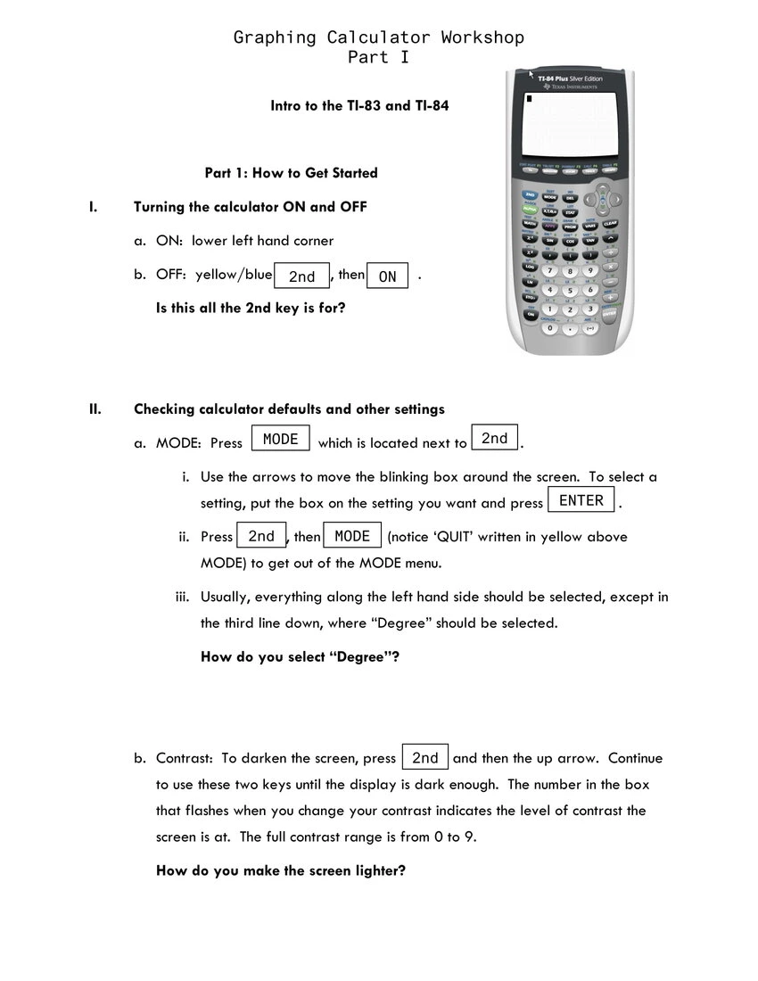
To power on your calculator, simply press the “ON” button, usually located in the bottom-left corner. Most calculators will display a “home” screen or a previous calculation. To turn it off, press “2nd” (or “Shift” depending on the model) followed by the “ON” button (which often doubles as “OFF”).

Navigation is primarily done using the directional arrow keys. These allow you to move the cursor on the screen, select menu options, or scroll through long lists of data or equations. The “ENTER” key confirms selections, while “CLEAR” or “DEL” removes input or closes screens. The “MODE” key is one of the most important – it opens a menu where you can set various parameters like angle units (degrees or radians), display format (normal, scientific, engineering), and graph type (function, parametric, polar, sequence). Always ensure your mode settings are appropriate for the problem you’re solving to avoid incorrect results.

Inputting Expressions and Performing Calculations

Inputting expressions on a graphing calculator is largely intuitive, similar to typing on a computer. Numbers and basic operations (+, -, *, /) are directly accessible. For powers, use the caret key (^). To input negative numbers, use the dedicated negative sign key ((-)), not the subtraction key (-), as they serve different functions. Parentheses () are vital for controlling the order of operations, just as in standard algebraic notation.

For example, to calculate (5 + 3) / 2, you would type ( 5 + 3 ) / 2 ENTER. To find the square root of 25, you’d typically press 2nd then the x^2 key (which often has √ above it), then 25 ENTER. Practice inputting various expressions to become comfortable with the syntax and ensure your results are accurate. Many calculators also have an “ANS” function (usually accessed via 2nd + (-)) which allows you to use the result of the previous calculation in your next one, streamlining multi-step problems.

Understanding Modes: Radian vs. Degree, Function vs. Parametric

The “MODE” settings are critical because they dictate how the calculator interprets and displays information.

• Angle Units (Radian vs. Degree): This is paramount for trigonometry. If you’re working with angles in degrees (e.g., a 45-degree angle), your calculator must be in DEGREE mode. If you’re using radians (e.g., π/2 radians), it must be in RADIAN mode. A common mistake is to perform trigonometric calculations in the wrong mode, leading to wildly inaccurate answers.
• Graph Type (Function, Parametric, Polar, Sequence):
  • Function Mode (Y=): The most common mode, used for plotting equations where Y is a function of X (e.g., Y = 2X + 3).
  • Parametric Mode: Used to graph equations where both X and Y are functions of a third variable, T (e.g., X = 2cos(T), Y = 2sin(T)).
  • Polar Mode: For graphing equations in polar coordinates (r and θ, e.g., r = 3sin(θ)).
  • Sequence Mode: For working with sequences, typically denoted as u(n).
• Display Format (Normal, Sci, Eng): Controls how numbers are displayed (e.g., 12345 vs. 1.2345E4).
• Decimal Places: Some calculators allow you to fix the number of decimal places displayed.

Regularly checking and adjusting the MODE settings based on the problem at hand will prevent countless errors and ensure the calculator behaves as expected.

Unlocking Visualization: Graphing Functions and Data

The true power of a graphing calculator lies in its ability to visualize mathematical relationships. This section explores how to plot functions, manipulate the viewing window, and extract meaningful insights from graphs.

Entering and Plotting Equations (Y= editor)

To graph a function, you typically navigate to the “Y=” editor (often a dedicated button). Here, you can enter multiple equations, usually as Y1=, Y2=, Y3=, etc. Use the “X, T, θ, n” key (which cycles through variables depending on your MODE) to input the independent variable.

For example, to graph Y = X^2 - 4:

1. Press the “Y=” button.
2. Navigate to Y1= (or an empty slot).
3. Type X^2 - 4.
4. Press the “GRAPH” button.

The calculator will then display the graph of the parabola. You can select or deselect equations in the “Y=” editor to hide or show them on the graph, which is useful for comparing multiple functions.

Adjusting the Viewing Window: Zoom and Window Settings

When you first graph an equation, the default viewing window might not show the most relevant parts of the graph. This is where “WINDOW” and “ZOOM” functions become invaluable.

• WINDOW: Pressing the “WINDOW” button allows you to manually set the Xmin, Xmax, Ymin, Ymax values, which define the boundaries of your graph’s display. You can also set Xscl and Yscl to determine the spacing of tick marks on the axes. Manually adjusting the window provides precise control over what you see.
• ZOOM: The “ZOOM” menu offers quick ways to adjust the window.
  • Zoom Standard (ZStandard): Resets the window to a default -10 to 10 range for both X and Y axes. A good starting point.
  • Zoom Fit (ZFit): Adjusts the Y-axis range to fit the current X-axis range, useful when you know your X-range but aren’t sure of the Y-values.
  • Zoom In/Out: Allows you to select a point on the graph and zoom in or out around it.
  • Zoom Box: Lets you draw a box around a specific area you want to magnify.

Mastering these functions is crucial for effectively analyzing graphs, ensuring you capture all relevant features like turning points, intercepts, and asymptotes.

Tracing, Intersections, and Roots: Analyzing Graphs

Once a graph is displayed, several powerful analytical tools become available, usually found under the “CALC” (Calculate) menu (accessed via 2nd + “TRACE”).

• Trace: Pressing the “TRACE” button allows you to move a cursor along the graph, displaying the X and Y coordinates at each point. This is useful for getting approximate values.
• Value: In the “CALC” menu, “Value” lets you input a specific X-value and the calculator will find the corresponding Y-value on the selected function.
• Roots (Zeros): This function finds where the graph intersects the X-axis (i.e., where Y = 0). You’ll typically be prompted to select a “Left Bound” and “Right Bound” (points to the left and right of the root) and then a “Guess” to help the calculator pinpoint the exact location.
• Intersection: Used to find the point(s) where two graphs cross. After selecting “Intersection,” you’ll be asked to select the “First Curve,” “Second Curve,” and a “Guess” near the intersection point.
• Minimum/Maximum: These functions locate the lowest or highest point (local minimum or maximum) of a curve within a specified interval, again using “Left Bound,” “Right Bound,” and “Guess” prompts.

These tools transform the calculator from a mere plotter into a powerful analytical instrument, enabling you to solve equations graphically, optimize functions, and understand critical points of mathematical models.

Plotting Data and Statistical Graphs

Beyond functions, graphing calculators excel at visualizing and analyzing data. This is particularly useful in statistics.

1. Enter Data: Access the “STAT” menu, then select “Edit” to open the list editor. Here, you can input data into columns (L1, L2, L3, etc.).
2. Set Up StatPlot: Go to “STAT PLOT” (usually 2nd + “Y=”). Turn on one of the plots (e.g., Plot1).
3. Choose Plot Type: Select the type of graph you want:
   • Scatter Plot: For showing the relationship between two variables (e.g., L1 vs. L2).
   • Line Plot: Similar to scatter but connects the points.
   • Histogram: For displaying the distribution of a single variable.
   • Box Plot (Box and Whisker): For showing median, quartiles, and outliers.
   • Normal Probability Plot: To assess if data is normally distributed.
4. Graph: Press “ZOOM,” then select “ZoomStat” (often option 9). This automatically adjusts the window to fit your data.

Graphing data visually helps in identifying trends, patterns, outliers, and the overall distribution of a dataset before performing formal statistical analysis.

Advanced Features for Enhanced Learning and Problem-Solving

While basic graphing and calculation are core functions, modern graphing calculators pack an array of advanced features that can tackle more sophisticated mathematical challenges, significantly aiding in higher-level courses and professional applications.

Solving Equations and Systems of Equations

Graphing calculators offer several methods to solve equations, moving beyond simply finding roots on a graph.

• Numerical Solver: Many calculators have an “Equation Solver” or “Numeric Solver” (often found under “MATH” or “APPS” menus). You input an equation (e.g., 0 = X^3 - 2X - 1) and provide a guess, and the calculator iteratively finds a numerical solution for X. This is particularly useful for complex equations that are difficult to solve algebraically.
• Systems of Equations (Matrix Method): For systems of linear equations (e.g., 2x + 3y = 7 and x - y = 1), you can represent them as matrices. The calculator’s matrix functions (usually under a dedicated “MATRIX” menu) allow you to enter the coefficient matrix and the constant matrix, then use inverse matrix operations (A^-1 * B) or row reduction (rref()) to find the solution vector.
• Graphical Intersection: As discussed earlier, plotting each equation as Y1= and Y2= and then using the “CALC -> Intersection” feature provides a visual and precise solution for two equations.

These methods streamline the process of solving equations, freeing up time to understand the underlying concepts rather than getting bogged down in algebraic manipulation.

Calculus Functions: Derivatives and Integrals

For students of calculus, graphing calculators are indispensable. They can perform both numerical differentiation and integration.

• Numerical Derivative (nDeriv): Found in the “MATH” menu, nDeriv( allows you to calculate the numerical derivative of a function at a specific point. The syntax is typically nDeriv(function, variable, value), e.g., nDeriv(X^2, X, 3) would give the derivative of X^2 at X=3.
• Numerical Integral (fnInt): Also in the “MATH” menu, fnInt( computes the definite integral of a function over a given interval. The syntax is fnInt(function, variable, lower_limit, upper_limit), e.g., fnInt(X^2, X, 0, 2) would calculate the definite integral of X^2 from 0 to 2.
• Graphical Derivatives/Integrals: Some advanced models can display the derivative function itself or shade the area under a curve directly on the graph, providing a visual interpretation of these calculus concepts.

It’s important to remember that these are numerical approximations. While incredibly accurate for most practical purposes, they are not symbolic derivatives or integrals (unless your calculator has a CAS, like the TI-Nspire CX CAS or HP Prime).

Matrix Operations and Linear Algebra

Graphing calculators are powerful tools for linear algebra, making matrix operations manageable even for large matrices.

• Entering Matrices: A dedicated “MATRIX” menu allows you to define and edit matrices by specifying dimensions (rows x columns) and entering elements.
• Matrix Arithmetic: Once matrices are defined, you can perform addition, subtraction, multiplication, and scalar multiplication directly.
• Advanced Operations: Calculators can compute determinants (det()), inverses (^-1), transposes (^T), and perform row reduction (rref()), which is essential for solving systems of equations and analyzing vector spaces.
• Eigenvalues/Eigenvectors: More advanced models might also offer functions to calculate eigenvalues and eigenvectors.

These matrix capabilities are invaluable for subjects like linear algebra, multivariable calculus, and various engineering and scientific applications.

Programming Your Calculator: Customizing Workflows

Many graphing calculators allow users to write and store programs, transforming them into specialized tools for repetitive or complex tasks. This feature lets you automate sequences of operations, create custom formulas, or even develop small games.

• Accessing the Program Editor: Usually found under a “PRGM” (Program) menu. Here you can create new programs or edit existing ones.
• Basic Commands: Programs are written using a simple scripting language, typically including commands for input (Input), output (Disp), conditional statements (If...Then...Else), loops (For, While), and calls to built-in functions.
• Applications: Common uses include:
  • Custom Formulas: A program to calculate quadratic formula roots.
  • Data Analysis: A program to sort lists or perform specific statistical tests.
  • Interactive Tools: Programs that guide users through a series of inputs to solve a specific problem.

Programming can significantly enhance efficiency and personalize your calculator’s functionality, making it an even more tailored and powerful academic or professional assistant.

Best Practices and Troubleshooting Tips

Even with advanced features, getting the most out of your graphing calculator requires good habits and the ability to troubleshoot common issues.

Maintaining Your Calculator: Battery Life and Storage

• Battery Management: Most graphing calculators use either AAA batteries or rechargeable lithium-ion batteries. Always carry spare batteries or ensure your rechargeable model is topped up before critical exams or long study sessions. Dimming the screen backlight (if available) can extend battery life.
• Storage: Keep your calculator in a protective case to prevent screen scratches and button damage. Avoid exposing it to extreme temperatures or moisture.
• Data Backup: Periodically back up important programs, lists, and matrices to your computer using the appropriate connectivity cable and software (e.g., TI Connect for Texas Instruments calculators). This safeguards your work against battery depletion or accidental resets.
• Regular Updates: Check the manufacturer’s website for operating system (OS) updates. These often include bug fixes, performance improvements, and sometimes new features.

Common Error Messages and Their Solutions

Encountering an error message can be frustrating, but understanding common ones can quickly resolve issues.

• SYNTAX ERROR: You’ve entered an invalid expression (e.g., missing parenthesis, incorrect function argument). Carefully review your input.
• DOMAIN ERROR: The input value is outside the function’s valid domain (e.g., taking the square root of a negative number, log(0)). Check your X-values or function definition.
• DIVIDE BY 0: Attempting to divide by zero. Review denominators in your expressions or check for asymptotes in graphs.
• INVALID DIM: Often occurs when performing matrix operations with incompatible dimensions (e.g., trying to add a 2×3 matrix to a 3×2 matrix).
• OVERFLOW ERROR: The result of a calculation is too large for the calculator to handle.
• MEMORY ERROR: The calculator doesn’t have enough free memory for the operation. Try clearing old programs or lists if not backed up.

When an error occurs, the calculator often highlights where the error is. Use the arrow keys to navigate to the error and correct it.

Utilizing Online Resources and Community Support

The graphing calculator community is vast and active. Don’t hesitate to seek help:

• Manufacturer Websites: Provide manuals, FAQs, OS updates, and sometimes tutorials.
• YouTube Tutorials: Many content creators offer step-by-step guides for specific calculator functions and models.
• Online Forums and Communities: Websites like Reddit (r/calculators, r/ti84), various math forums, and dedicated calculator enthusiast sites are excellent places to ask questions, share tips, and find solutions to complex problems.
• Textbook Resources: Many math textbooks include sections on using graphing calculators relevant to the course material.

By embracing these best practices and leveraging available support, your graphing calculator can become an even more reliable and powerful ally in your academic and professional journey. Far from being obsolete, it remains a cornerstone of practical technology for anyone engaging with complex numerical and graphical analysis.

aViewFromTheCave is a participant in the Amazon Services LLC Associates Program, an affiliate advertising program designed to provide a means for sites to earn advertising fees by advertising and linking to Amazon.com. Amazon, the Amazon logo, AmazonSupply, and the AmazonSupply logo are trademarks of Amazon.com, Inc. or its affiliates. As an Amazon Associate we earn affiliate commissions from qualifying purchases.