how do i find the function of a graph

Unraveling the algebraic expression behind a visual graph is a fundamental skill in mathematics, science, engineering, and data analysis. It bridges the gap between abstract visual representations and precise mathematical models. Whether you’re confronted with a scatter plot of experimental data or a geometric curve, understanding how to deduce its underlying function is crucial for prediction, analysis, and further computation. This process often involves a combination of visual pattern recognition, application of mathematical principles, and leveraging powerful digital tools.

Table of Contents

Understanding the Basics: Visual Clues and Common Forms

Before diving into complex techniques, recognizing the basic shapes and characteristics of common functions is the first step. Many real-world phenomena can be approximated by these fundamental forms, making visual inspection a powerful initial approach.

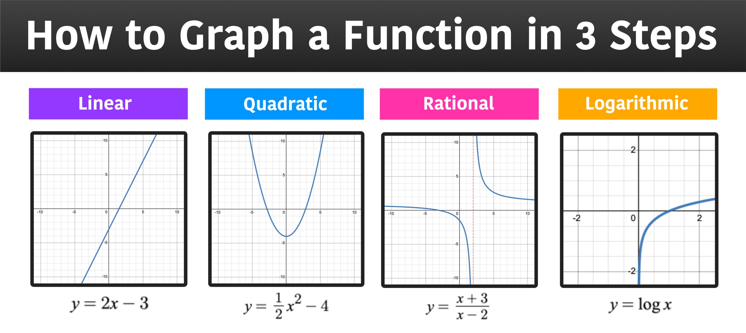
Linear Functions (y = mx + b)

A straight line on a graph always represents a linear function. The key characteristics to look for are a constant rate of change.

Identification: The graph is a straight line.
Parameters:
- Slope (m): Represents the steepness of the line. It can be calculated as “rise over run” (Δy / Δx) between any two distinct points on the line. A positive slope indicates an upward trend, a negative slope a downward trend, and a zero slope a horizontal line.
- Y-intercept (b): The point where the line crosses the y-axis (where x = 0).
Method: Choose two clear points (x₁, y₁) and (x₂, y₂) from the graph. Calculate the slope m = (y₂ - y₁) / (x₂ - x₁). Once m is known, substitute one point and m into the equation y = mx + b to solve for b.

Quadratic Functions (y = ax² + bx + c)

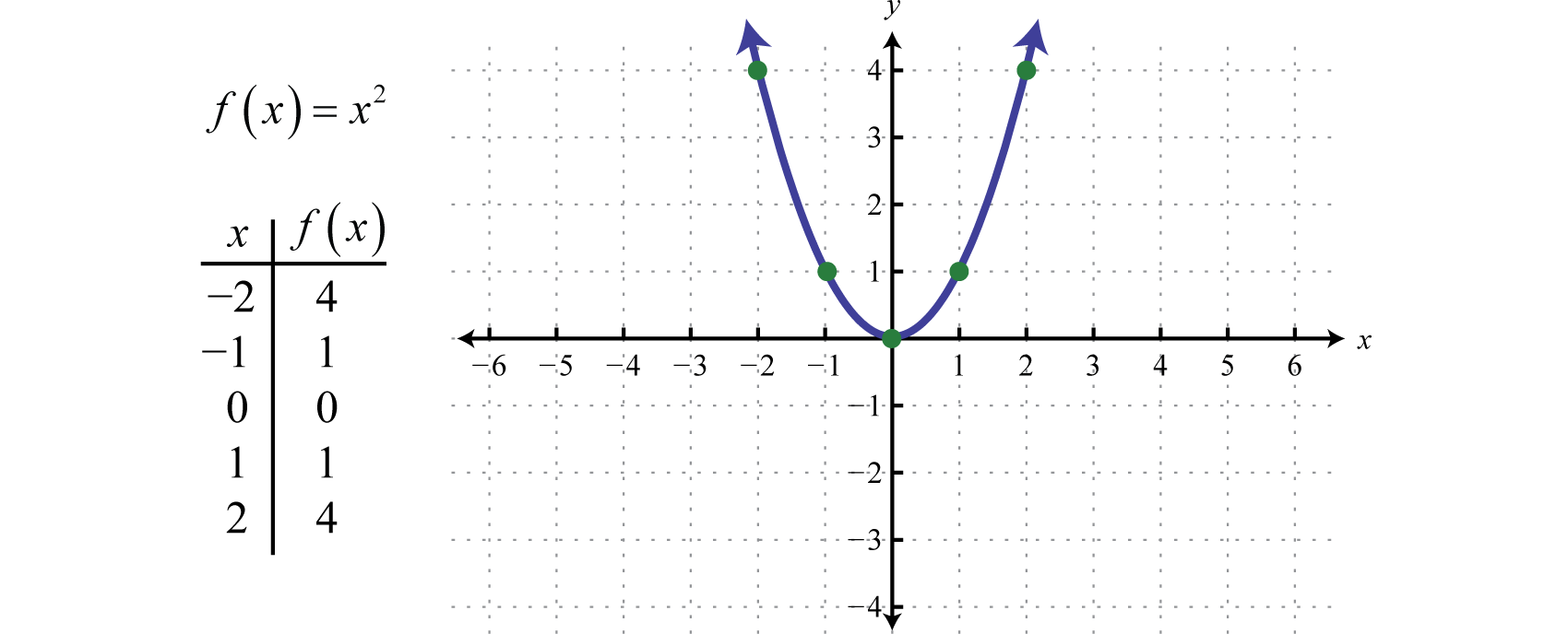
Quadratic functions create parabolas, distinctive U-shaped or inverted U-shaped curves.

Identification: The graph is a parabola, symmetric around a vertical axis. It has a single turning point (vertex) which is either a maximum or a minimum.
Parameters: The sign of ‘a’ determines the direction: a > 0 for an upward-opening parabola, a < 0 for a downward-opening one.
Method:
1. Vertex Form: If the vertex (h, k) is easily identifiable, the function can be written as y = a(x - h)² + k. Find another point (x, y) on the parabola and substitute it along with (h, k) into the vertex form to solve for ‘a’.
2. Intercept Form: If the x-intercepts (roots) p and q are clear, use y = a(x - p)(x - q). Again, use another point to find ‘a’.
3. Standard Form: If three non-collinear points are known, substitute them into y = ax² + bx + c to create a system of three linear equations with three unknowns (a, b, c), which can then be solved.

Exponential Functions (y = abˣ)

Exponential functions describe growth or decay patterns where the rate of change is proportional to the current value.

Identification: The graph exhibits rapid increase or decrease, often curving sharply and approaching a horizontal asymptote (a line it gets infinitely close to but never touches). It never passes through the x-axis unless shifted vertically.
Parameters: ‘a’ is the initial value (y-intercept when x=0), and ‘b’ is the base, representing the growth/decay factor.
Method:
1. Y-intercept: Identify the y-intercept (0, a). This gives you ‘a’.
2. Second Point: Choose another clear point (x, y). Substitute ‘a’, x, and y into y = a * bˣ and solve for b. For instance, if y = a * b² and a is known, then b = sqrt(y/a).

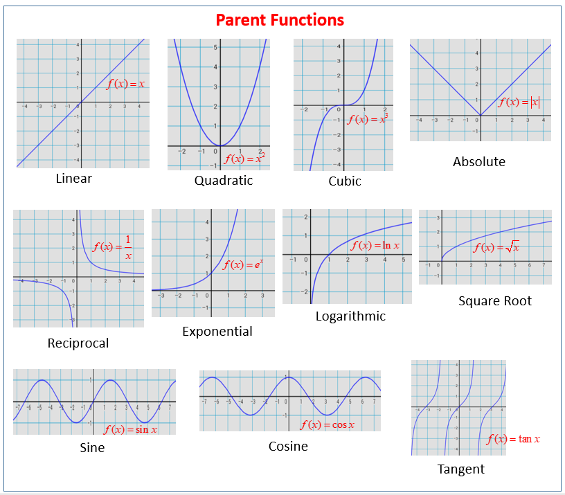
Other Common Forms (Logarithmic, Trigonometric, Power)

Logarithmic Functions: These are inverses of exponential functions, characterized by a vertical asymptote and a gradual increase/decrease. They often appear as y = a log_b(x - h) + k.
Trigonometric Functions (e.g., Sine, Cosine): These exhibit periodic, wave-like patterns. Look for amplitude, period, phase shift, and vertical shift to determine parameters in forms like y = A sin(Bx + C) + D.
Power Functions (y = axⁿ): These include parabolas (n=2), cubic curves (n=3), and hyperbolas (n=-1). They pass through the origin if n > 0 and are symmetric or antisymmetric depending on n.

Leveraging Digital Tools for Pattern Recognition and Regression

While visual inspection is helpful, for real-world data or complex curves, digital tools become indispensable. These tools can plot data, identify underlying patterns, and perform rigorous statistical analysis to find the best-fit function.

Online Graphing Calculators (Desmos, GeoGebra)

These interactive platforms are excellent for visualizing data, experimenting with different function types, and performing basic regression.

Desmos:
1. Data Input: Enter your data points (x₁, y₁), (x₂, y₂), etc., usually as a table.
2. Visual Fitting: Type in a general form of a function (e.g., y = mx + b for linear, y = ax^2 + bx + c for quadratic).
3. Regression: To perform regression, use a tilde ~ instead of an equals sign =. For example, for linear regression, type y₁ ~ mx₁ + b. Desmos will automatically calculate the best-fit m and b values and display the regression line. Similarly, y₁ ~ ax₁^2 + bx₁ + c will provide quadratic regression parameters.
4. Experimentation: Easily adjust parameters with sliders to see how they affect the graph, helping you visually align a function with your data points.
GeoGebra: Offers similar functionalities with a robust suite of geometric, algebraic, and calculus tools. You can input data, define functions, and use built-in regression commands to find the equation of a trend line.

Statistical Software and Programming Libraries (Excel, Python, R)

For more complex datasets or professional analysis, dedicated statistical software and programming environments provide advanced regression capabilities.

Microsoft Excel:
1. Scatter Plot: Create a scatter plot of your x and y data.
2. Add Trendline: Right-click on the data points in the chart and select “Add Trendline.”
3. Choose Function Type: Excel offers various trendline options: Linear, Exponential, Logarithmic, Polynomial (quadratic, cubic, etc.), Power, and Moving Average.
4. Display Equation: Crucially, check the box “Display Equation on chart” to see the function Excel has calculated. You can also display the R-squared value, which indicates how well the model fits the data (closer to 1 is better).
Python (with libraries like NumPy, SciPy, Matplotlib, Pandas):
1. Data Handling: Use Pandas to import and manage your data.
2. Visualization: Matplotlib can create scatter plots.
3. Numerical Operations: NumPy is essential for numerical computations, including polynomial fitting. numpy.polyfit(x, y, degree) can directly return the coefficients of a polynomial of a specified degree that best fits the data.
4. Optimization: SciPy’s scipy.optimize.curve_fit is a powerful tool for fitting arbitrary user-defined functions to data, allowing for highly flexible modeling beyond standard polynomials. You define your function (e.g., def func(x, a, b, c): return a * np.exp(b * x) + c), provide initial guesses for parameters, and curve_fit will find the optimal parameters.
R: A statistical programming language with extensive packages for data analysis.
1. Data Import: Read data into data frames.
2. Linear Models: lm() function for linear regression.
3. Non-Linear Models: nls() function for non-linear least squares fitting, allowing you to specify a formula and initial parameter estimates.

AI-Powered Solutions (Wolfram Alpha, Symbolab)

For quick solutions or verification, these computational knowledge engines can often identify functions from given points or descriptions.

Wolfram Alpha: You can input data points directly (e.g., fit (1,2), (3,4), (5,6)) and it will attempt to find the simplest function that passes through or approximates those points. You can also specify the type of function (e.g., linear fit (1,2), (3,4)).
Symbolab: Offers similar functionalities, particularly for symbolic mathematics, allowing you to enter points and often get a step-by-step solution for finding the function’s equation.

The Process: From Data Points to Functional Expression

Finding the function of a graph, especially from a set of discrete data points, is an iterative and analytical process.

Identifying Key Points and Symmetries

Intercepts: The x-intercepts (where y=0) and y-intercept (where x=0) are often crucial for determining constants or factors.
Turning Points: Maxima and minima (vertices for parabolas, peaks/troughs for waves) provide information about the function’s derivative and overall shape.
Asymptotes: Horizontal, vertical, or oblique asymptotes indicate specific functional behaviors (e.g., rational functions, exponential functions).
Symmetry:
- Y-axis symmetry: If f(x) = f(-x), the function is even (e.g., y = x², y = cos(x)).
- Origin symmetry: If f(-x) = -f(x), the function is odd (e.g., y = x³, y = sin(x)).
- Periodicity: For trigonometric functions, identifying the period is vital.

Testing Hypotheses and Iterative Refinement

Based on visual inspection and key points, form hypotheses about the type of function.

Initial Guess: “This looks like a quadratic.”
Parameter Estimation: Estimate initial parameters (e.g., vertex, x-intercepts).
Formulate Equation: Write down the hypothesized function with these parameters.
Test with Data: Plug in other data points from the graph into your hypothesized function. How closely do the predicted values match the actual values?
Refine: Adjust parameters or even switch to a different function type if the fit is poor. For instance, if a linear fit isn’t good, try a quadratic or exponential. This process is highly interactive when using graphing software.

Regression Analysis: The Quantitative Approach

When dealing with noisy or approximate data, regression analysis provides a statistical method to find the “best-fit” function. It minimizes the distance (usually the sum of squared residuals) between the function’s predicted values and the actual observed data points.

Least Squares Method: The most common method, it finds the line or curve that minimizes the sum of the squares of the vertical distances from each data point to the line/curve.
R-squared Value: This statistical measure (ranging from 0 to 1) indicates the proportion of variance in the dependent variable that can be predicted from the independent variable(s). A higher R-squared value means a better fit.
Residual Analysis: Examining the residuals (the differences between observed and predicted y-values) can reveal if the chosen function type is appropriate. A random scatter of residuals suggests a good fit, while patterns (e.g., a curve in the residuals) indicate that a different function type might be better.

Advanced Techniques and Considerations

Beyond basic function fitting, more sophisticated scenarios require a deeper understanding of mathematical modeling.

Piecewise Functions and Domain Restrictions

Sometimes, a single function cannot accurately represent the entire graph. In such cases, the graph might be composed of different function segments, each valid over a specific domain.

Identification: Look for sharp corners, sudden changes in slope, or discontinuities.
Method: Break the graph into sections where a single function type seems to fit. Define each function and its corresponding domain (e.g., f(x) = x for x < 0 and f(x) = x² for x ≥ 0).

Parameter Optimization and Curve Fitting

For highly complex functions or when you have a theoretical model with several parameters, advanced optimization algorithms are used.

Non-linear Least Squares: For functions that are non-linear in their parameters (e.g., y = A*e^(Bx) + C), iterative algorithms adjust the parameters to minimize the sum of squared errors. This is what functions like scipy.optimize.curve_fit do.
Goodness of Fit: Beyond R-squared, metrics like AIC (Akaike Information Criterion) or BIC (Bayesian Information Criterion) help in model selection, especially when comparing models with different numbers of parameters.

Real-World Data Challenges

Real-world data is rarely perfect.

Noise: Data often contains random fluctuations or measurement errors. Regression aims to find the underlying trend despite this noise.
Outliers: Extreme data points that deviate significantly from the general trend can heavily influence the fit. Identify and carefully consider whether to remove or adjust them.
Extrapolation vs. Interpolation: Using a fitted function to predict values within the observed data range (interpolation) is generally safer than predicting values outside that range (extrapolation), which carries higher uncertainty.

By combining visual intuition with the power of digital tools and a solid understanding of mathematical principles, you can effectively find the function of a graph, transforming raw data or visual patterns into actionable mathematical models.

aViewFromTheCave is a participant in the Amazon Services LLC Associates Program, an affiliate advertising program designed to provide a means for sites to earn advertising fees by advertising and linking to Amazon.com. Amazon, the Amazon logo, AmazonSupply, and the AmazonSupply logo are trademarks of Amazon.com, Inc. or its affiliates. As an Amazon Associate we earn affiliate commissions from qualifying purchases.