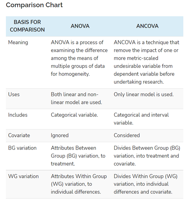
ANCOVA, or Analysis of Covariance, is a powerful statistical technique that extends the familiar Analysis of Variance (ANOVA) by incorporating one or more continuous covariates. While ANOVA is excellent for examining differences in a dependent variable across different groups (defined by categorical independent variables), ANCOVA allows researchers to account for the influence of other continuous variables that might also affect the dependent variable. This makes ANCOVA a more sophisticated tool for isolating the true effects of the independent variables of interest, leading to more precise and robust conclusions.
In essence, ANCOVA “adjusts” the group means of the dependent variable based on the values of the covariate. Imagine you’re studying the effectiveness of different teaching methods on student test scores. A simple ANOVA would compare the average scores across the teaching methods. However, pre-existing student intelligence (measured by an IQ score) could also significantly impact test scores, regardless of the teaching method. ANCOVA allows you to statistically control for these pre-existing differences in IQ, giving you a clearer picture of how each teaching method truly impacts scores, independent of initial intelligence levels.

The strength of ANCOVA lies in its ability to increase statistical power. By reducing the unexplained variance in the dependent variable (the variance attributable to the covariate), ANCOVA can make it easier to detect statistically significant differences between groups that might otherwise be masked by the covariate’s influence. This is particularly valuable in fields like psychology, education, medicine, and social sciences, where complex interactions between variables are common.
The Foundation: Understanding ANOVA’s Limitations
Before diving into ANCOVA, it’s crucial to understand the limitations of its predecessor, ANOVA. ANOVA is a cornerstone of statistical analysis, designed to compare the means of a dependent variable across two or more independent groups. For instance, if we want to see if a new drug has a different effect on blood pressure compared to a placebo, we’d use ANOVA to compare the average blood pressure readings in the drug group and the placebo group.
ANOVA works by partitioning the total variance in the dependent variable into components attributable to the independent variable (between-group variance) and components due to random error or other unmeasured factors (within-group variance). A significant F-statistic indicates that the differences in means between the groups are unlikely to have occurred by chance.
However, ANOVA assumes that all other factors influencing the dependent variable are either constant across groups or are randomly distributed. In real-world research, this is often not the case. Many extraneous variables can covary with the dependent variable and also differ across the groups, even if they are not the primary focus of the study. These confounding variables can inflate the within-group variance, making it harder to detect real differences between the groups.
Consider the blood pressure example again. What if the participants in the drug group were, on average, older than those in the placebo group? Age is known to influence blood pressure. If we don’t account for this difference in age, the observed difference in blood pressure between the groups might be partly due to the drug and partly due to the age disparity. ANOVA, in its basic form, cannot disentangle these effects. This is where ANCOVA steps in to provide a more nuanced analysis.
The Need for Control in Experimental Design
Experimental design is all about isolating the effect of an independent variable on a dependent variable. Researchers strive to create conditions where only the variable being manipulated differs between groups, while all other potentially influential factors remain constant or are balanced out. However, perfect control is rarely achievable.
Random assignment helps to equalize groups on many known and unknown variables at the start of an experiment. But even with randomization, there can be systematic differences between groups, especially in observational studies or when participants cannot be perfectly matched. For example, in a study comparing the effectiveness of two educational interventions, students might enter the study with varying levels of prior knowledge. If one group, by chance, has a higher average prior knowledge, it could confound the results.
The goal of statistical control is to mimic the ideal experimental scenario where extraneous variables are held constant. ANCOVA achieves this by statistically adjusting the dependent variable scores. It essentially estimates what the group means would be if all groups had the same average score on the covariate. This adjustment removes the variance in the dependent variable that is predictable from the covariate, thereby clarifying the unique effect of the independent variable.
Variance Explained and Unexplained
In any statistical analysis, the total variation observed in the dependent variable can be broadly categorized into two parts: variance that is explained by the model (i.e., by the independent variables and covariates) and variance that is unexplained (i.e., residual error).
ANOVA focuses on explaining variance based solely on categorical independent variables. The F-statistic in ANOVA is a ratio of the variance explained by the groups (between-group variance) to the unexplained variance (within-group variance). A higher ratio suggests that the group differences are substantial relative to the random noise.
ANCOVA builds upon this by including one or more covariates. The model now explains variance in the dependent variable from both the categorical independent variable(s) and the continuous covariate(s). The key benefit is that the variance explained by the covariate is removed from the unexplained variance. This effectively “cleans up” the error term, making the between-group variance appear larger in proportion to the remaining error. Consequently, the F-statistic for the independent variable of interest becomes more sensitive, increasing the likelihood of detecting a statistically significant effect if one truly exists.
The Mechanics of ANCOVA: How It Works
ANCOVA integrates the principles of regression analysis with ANOVA. At its core, ANCOVA estimates a regression model where the dependent variable is predicted by both the categorical independent variable(s) and the continuous covariate(s). The statistical significance tests are then performed on the independent variable(s), after accounting for the contribution of the covariate(s).
Let’s consider a simple ANCOVA with one categorical independent variable (Factor A with groups A1, A2, A3) and one continuous covariate (X). The model can be conceptualized as follows:
$Y = beta0 + tauA + beta_1 X + epsilon$
Where:
- $Y$ is the dependent variable.
- $beta_0$ is the overall intercept.
- $tau_A$ represents the effect of the different levels of Factor A.
- $beta_1$ is the regression coefficient for the covariate X, indicating how much Y changes for a one-unit increase in X, holding Factor A constant.
- $epsilon$ is the error term.
The ANCOVA procedure essentially performs a regression of Y on X and the dummy variables representing Factor A. It then tests whether the coefficients associated with the dummy variables for Factor A are significantly different from zero, after the effect of X has been accounted for. Alternatively, ANCOVA can be viewed as adjusting the raw group means by adding back the predicted effect of the covariate for the average covariate value across all groups. This results in adjusted means, which are then compared using an ANOVA-like procedure.
Assumptions of ANCOVA
Like any statistical test, ANCOVA relies on several assumptions for its results to be valid. Violations of these assumptions can lead to misleading conclusions.
- Independence of Observations: The observations within and between groups should be independent. This is a fundamental assumption for most statistical tests.
- Normality of Residuals: The residuals (the differences between observed and predicted values) should be approximately normally distributed. This is important for the validity of the F-tests.
- Homogeneity of Variances (Homoscedasticity): The variance of the residuals should be roughly equal across all groups. This is similar to the assumption in ANOVA.
- Linearity of Relationship: There should be a linear relationship between the dependent variable and the covariate within each group. This is a critical assumption for ANCOVA. Researchers often check this by plotting the dependent variable against the covariate separately for each group.
- Homogeneity of Regression Slopes (Parallel Slopes Assumption): This is the most crucial assumption specific to ANCOVA. It posits that the slope of the regression line relating the dependent variable to the covariate is the same for all groups of the independent variable. In other words, the effect of the covariate on the dependent variable does not differ across the groups. If this assumption is violated, the ANCOVA model is inappropriate, and alternative analyses (e.g., including an interaction term between the covariate and the independent variable) are needed.
Researchers typically assess these assumptions using diagnostic plots (e.g., residual plots, Q-Q plots) and statistical tests (e.g., Levene’s test for homogeneity of variances, tests for interaction effects).
The Role of the Covariate
The covariate is a continuous variable that is thought to influence the dependent variable and may differ across the groups of the independent variable. The primary purpose of including a covariate is to reduce the error variance. By accounting for the variation in the dependent variable that can be explained by the covariate, ANCOVA can increase the statistical power of the test for the independent variable of interest.
Selecting an appropriate covariate is crucial. It should be:
- Relevant: The covariate should have a theoretical or empirical link to the dependent variable.
- Measured Reliably: Any measurement error in the covariate can attenuate its effectiveness in reducing error variance.
- Not affected by the treatment: The covariate should ideally be measured before the independent variable has had a chance to influence it. This is a strong assumption and often where pre-tests are used as covariates. If the covariate is affected by the treatment, then its inclusion might lead to biased results.
Common examples of covariates include pre-test scores in educational studies, baseline measurements of a physiological variable in medical research, or pre-existing individual characteristics like age or IQ in psychological experiments.
When to Use ANCOVA: Practical Applications
ANCOVA is a versatile statistical tool employed across various disciplines whenever researchers need to compare group means while statistically controlling for the influence of one or more continuous variables. Its application is particularly widespread in fields that often deal with complex causal pathways and where perfect experimental control is challenging.
One of the most common scenarios for ANCOVA is in educational research. For instance, if a researcher wants to evaluate the effectiveness of a new teaching method compared to a traditional one on students’ final exam scores, they would typically measure students’ prior knowledge of the subject (e.g., a pre-test score) as a covariate. By using ANCOVA, the researcher can adjust for any initial differences in knowledge levels between the groups. This allows for a more accurate assessment of the true impact of the teaching method itself. If students in the new method group happened to have slightly higher pre-test scores, ANCOVA would statistically “level the playing field” before comparing the final exam scores.
In clinical trials and medical research, ANCOVA is frequently used to analyze the efficacy of different treatments. For example, when comparing the effect of two different pain management strategies on reported pain levels, researchers might use a baseline pain score (measured before the intervention) as a covariate. This helps to account for individual differences in pain sensitivity or the severity of the condition at the outset. Similarly, a study comparing the impact of different diets on weight loss might use baseline body weight as a covariate.
Psychological research also benefits greatly from ANCOVA. If a psychologist is investigating the effectiveness of a new therapy for reducing anxiety, they might use a baseline anxiety score as a covariate when comparing the anxiety levels of participants receiving the new therapy versus a control group. This ensures that any observed reduction in anxiety is attributable to the therapy and not just pre-existing lower levels of anxiety.
Improving Statistical Power
A primary motivation for using ANCOVA is to increase the statistical power of the analysis. Statistical power refers to the probability of correctly rejecting a false null hypothesis – essentially, the ability of a test to detect a real effect if one exists.
In ANOVA, the total variance is partitioned into variance explained by the independent variable and error variance. If there are uncontrolled sources of variation in the dependent variable that also differ across groups, these will contribute to the error variance. A larger error variance can mask a real effect of the independent variable, leading to a non-significant result even when a treatment has a true effect.
By including a covariate that is significantly correlated with the dependent variable, ANCOVA can explain a portion of this error variance. This effectively reduces the residual error variance. When the error variance is smaller, the F-statistic (which is a ratio of variance explained by the treatment to the error variance) becomes larger, assuming the treatment effect remains constant. A larger F-statistic increases the likelihood of achieving statistical significance, thus enhancing the study’s power to detect a true effect.
For instance, consider a study comparing two exercise programs on cardiovascular fitness. If participants naturally vary widely in their initial fitness levels, and this variation is not accounted for, the differences between the exercise programs might be obscured by the pre-existing fitness disparities. By using a pre-program fitness measure as a covariate, ANCOVA can isolate the effect of each program more effectively, potentially revealing a significant difference that might have been missed by a simple ANOVA.
Addressing Confounding Variables
In observational studies or quasi-experimental designs, it is often impossible to randomly assign participants to groups. This can lead to systematic differences between groups on variables that are not of primary interest but could influence the outcome. These are known as confounding variables.
ANCOVA provides a statistical method to control for these confounding variables, effectively adjusting for their influence. By including a confounding variable as a covariate, the analysis estimates the relationship between the independent variable and the dependent variable as if the groups were equal on the confounding variable. This helps to mitigate bias and provides a more accurate estimate of the true effect of the independent variable.
For example, imagine a study examining the effect of a company’s new management training program on employee productivity. If employees in the training group also happen to be younger on average than those in the control group, and age is known to correlate with productivity, then age is a confounder. ANCOVA can be used with age as a covariate to adjust for this age difference, allowing for a clearer assessment of the training program’s impact. Without this adjustment, the observed increase in productivity might be partly attributed to the training and partly to the younger age of the participants.
Potential Pitfalls and Advanced Considerations
While ANCOVA is a powerful tool, its effective application requires careful attention to its underlying assumptions and potential complexities. Misapplication or misunderstanding of ANCOVA can lead to incorrect conclusions.
One of the most critical assumptions, as mentioned, is the homogeneity of regression slopes. If the relationship between the covariate and the dependent variable differs across the groups, simply including the covariate as a main effect in the ANCOVA model is inappropriate. This is because the model assumes a single regression slope for all groups. When this assumption is violated, it implies that the effect of the covariate itself is moderated by the independent variable. In such cases, an interaction term between the independent variable and the covariate should be included in the model. This interaction term allows for different regression slopes for each group, providing a more accurate representation of the data. Detecting and addressing this violation is paramount for valid ANCOVA results.
Another common issue arises from the choice and measurement of the covariate. An ineffective covariate is one that is not sufficiently correlated with the dependent variable. If the covariate explains little of the variance in the dependent variable, it will do little to reduce the error variance, and the potential gains in statistical power will be minimal. Conversely, a covariate that is susceptible to measurement error can actually attenuate the results, making it harder to detect a true effect. The relevance and reliability of the covariate are thus paramount.
Furthermore, ANCOVA assumes that the covariate is not influenced by the independent variable. If the independent variable (e.g., a treatment) can affect the covariate, then using that covariate in ANCOVA can lead to biased results. For instance, if the dependent variable is post-treatment scores, and the covariate is a measure that is also affected by the treatment, then the ANCOVA might incorrectly attribute some of the treatment effect to the covariate. In such situations, pre-treatment measures of the covariate are typically preferred.
Dealing with Violations of Assumptions
When ANCOVA’s assumptions are violated, researchers have several options. For the homogeneity of regression slopes assumption, the most common solution is to include an interaction term between the covariate and the independent variable. If this interaction is statistically significant, it indicates that the effect of the covariate differs across groups, and the standard ANCOVA model is inappropriate. The interpretation then shifts to understanding how the covariate’s effect varies by group.
If the assumption of homogeneity of variances is violated, transformations of the dependent variable or the use of robust statistical methods might be considered. Similarly, if residuals are not normally distributed, especially with smaller sample sizes, non-parametric alternatives or bootstrapping techniques could be explored. However, ANCOVA is generally considered to be relatively robust to moderate violations of normality and homogeneity of variances, particularly with larger sample sizes.
The issue of the covariate being affected by the treatment is more complex. If a pre-test is used as a covariate and there is significant treatment effect, it can lead to “regression to the mean” artifacts and adjusted means that are difficult to interpret. This is where careful study design and advanced modeling techniques, such as latent growth curve modeling, might be more appropriate.

ANCOVA with Multiple Covariates
ANCOVA can be extended to include multiple covariates, a technique known as Multiple Analysis of Covariance (MANCOVA). This allows researchers to control for the influence of several continuous variables simultaneously. MANCOVA is particularly useful when multiple factors are known to affect the dependent variable.
For example, in a study evaluating the effectiveness of an educational intervention on student learning, one might include both pre-test scores and students’ reported motivation levels as covariates. MANCOVA would adjust the group means for both of these factors simultaneously. This can lead to even greater reductions in error variance and an increase in statistical power compared to using a single covariate.
However, using multiple covariates introduces additional complexities. The relationships between all variables (dependent variable, independent variables, and all covariates) become important. Assumptions such as linearity and homogeneity of regression slopes need to hold for each covariate. Furthermore, multicollinearity among the covariates (i.e., high correlation between covariates) can also pose problems for the stability and interpretability of the model. Researchers need to carefully consider the theoretical relevance of each covariate and examine their interrelationships before including them in a MANCOVA model. The interpretation of results in MANCOVA also becomes more intricate, as one is considering the effects after accounting for a multivariate set of influences.
aViewFromTheCave is a participant in the Amazon Services LLC Associates Program, an affiliate advertising program designed to provide a means for sites to earn advertising fees by advertising and linking to Amazon.com. Amazon, the Amazon logo, AmazonSupply, and the AmazonSupply logo are trademarks of Amazon.com, Inc. or its affiliates. As an Amazon Associate we earn affiliate commissions from qualifying purchases.