In the rapidly evolving landscape of technology, the performance of an application is often judged by its speed. We praise software that responds in milliseconds and criticize platforms that lag. However, beneath the surface of execution time lies a equally critical, yet often overlooked, dimension of computational efficiency: Space Complexity. While “Time Complexity” tells us how long an algorithm will take to run, “Space Complexity” tells us how much memory it needs to breathe.
As software systems scale to handle billions of users and massive datasets, understanding the memory footprint of our code is no longer just an academic exercise. It is a fundamental requirement for building scalable, cost-effective, and high-performing technology.

Decoding the Fundamentals: What is Space Complexity?
At its core, space complexity is a measure of the amount of working memory (RAM) an algorithm needs to run to completion as a function of the size of the input. In the era of modern computing, where multi-terabyte drives are common, it is tempting to think that memory is an infinite resource. However, in professional software development—especially in cloud computing, mobile app development, and embedded systems—memory remains a constrained and costly asset.
Defining Space Complexity in the Algorithmic Context
Space complexity encompasses all the memory required by an algorithm during its execution. This includes the memory needed for the input values, the memory for local variables, and the overhead of the instruction sequence. When we analyze an algorithm, we aren’t looking for a byte-perfect measurement, but rather a mathematical trend. We want to know: if the input size doubles, how does the memory requirement grow? Does it stay the same, does it double, or does it increase exponentially?
The Distinction Between Auxiliary Space and Total Space
A common point of confusion for many junior developers is the difference between “Auxiliary Space” and “Total Space Complexity.”
- Auxiliary Space refers specifically to the extra or temporary space used by the algorithm, excluding the space taken by the input itself.
- Total Space Complexity includes both the auxiliary space and the space occupied by the input.
In technical interviews and high-level system design, engineers often focus on auxiliary space because it represents the efficiency of the algorithm’s logic rather than the size of the data being processed. For instance, an in-place sorting algorithm is highly prized because its auxiliary space is constant, even if it is sorting a billion-record database.
Measuring Efficiency: How to Calculate Space Complexity
To calculate space complexity, we must look at the variables, data structures, and function calls within a program. Much like time complexity, we express this using Big O Notation, which provides a high-level abstraction of growth rates.
Fixed Space Requirements
Every program has a “Fixed Part” that is independent of the input size. This includes:
- Instruction Space: The memory required to store the compiled code.
- Simple Variables: Memory for constants and fixed-size variables (e.g., a single integer used as a loop counter).
- Fixed-size Structures: Any array or object that does not change size based on the input.
Because these elements do not grow with the input, they are considered $O(1)$ or “Constant Space.”
Variable Space Requirements and Big O Notation
The “Variable Part” is where space complexity becomes dynamic. This includes:
- Dynamic Memory Allocation: Creating arrays, lists, or trees whose size depends on the input $n$.
- Recursion Stacks: This is a silent killer of memory efficiency. Every time a function calls itself, a new “frame” is pushed onto the call stack, storing local variables and the return address. A recursive function that goes $n$ levels deep will have a space complexity of at least $O(n)$, even if it doesn’t explicitly create any large data structures.
To determine the Big O, we identify the fastest-growing term. If an algorithm uses a constant amount of extra memory plus an array of size $n$, the space complexity is $O(n)$.
Common Space Complexity Classes in Modern Programming
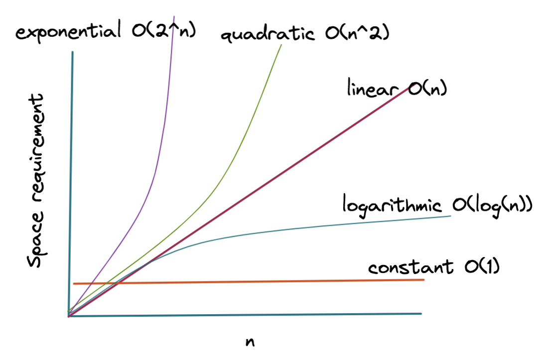
Understanding the different classes of space complexity allows developers to predict how their software will behave under heavy loads.
Constant Space: $O(1)$
This is the gold standard of space efficiency. An algorithm has $O(1)$ space complexity if the memory it uses does not change regardless of the input size.
- Example: A function that takes an array of any size and returns the sum of its elements. The function only needs a single “sum” variable to track the total, regardless of whether the array has ten elements or ten million.
Linear Space: $O(n)$
In linear space, the memory requirement grows in direct proportion to the input size.
- Example: Making a copy of an array. If you have an input list of $n$ items and you create a new list to store a modified version of those items, you are using $O(n)$ space. Most non-in-place algorithms fall into this category.
Logarithmic and Quadratic Space
- Logarithmic Space ($O(log n)$): Often seen in efficient recursive algorithms like Binary Search (when implemented recursively). The stack depth only increases by one for every doubling of the input size.
- Quadratic Space ($O(n^2)$): This is common in algorithms that involve 2D grids or matrices derived from a linear input. For example, if an algorithm creates a comparison matrix for a string of length $n$, it will require $n times n$ units of space. In the tech world, $O(n^2)$ space is often a red flag for scalability issues.
The Engineering Trade-off: Balancing Time and Space Complexity
In the real world of software engineering, we rarely get the best of both worlds. The “Time-Space Trade-off” is a fundamental concept where we sacrifice memory to gain speed, or vice versa.
Real-World Scenarios for Space Optimization
Consider Memoization, a technique used in dynamic programming. To speed up a calculation, we store the results of expensive function calls in a cache (using $O(n)$ space). The next time the same input occurs, we look it up in the cache (O(1) time) instead of recalculating it. Here, we are intentionally increasing space complexity to dramatically reduce time complexity.
Conversely, in Embedded Systems or IoT devices, memory is extremely limited. A developer might choose a slower algorithm that uses $O(1)$ space over a faster one that uses $O(n)$ space because the hardware literally cannot support the larger memory footprint.
Why Space Complexity Still Matters in the Age of Cheap Memory
It is a common misconception that “RAM is cheap, so space complexity doesn’t matter.” In a professional tech environment, this is false for three reasons:
- Cache Locality: Modern CPUs use caches (L1, L2, L3) that are much faster than RAM. Smaller memory footprints fit better in these caches, leading to significantly faster execution times.
- Cloud Costs: In cloud environments like AWS or Azure, you pay for the instance size. High memory usage forces you to use larger, more expensive instances, directly impacting the company’s bottom line.
- Garbage Collection Overhead: In languages like Java, Python, or Go, high memory usage triggers frequent “Garbage Collection” cycles, which can pause the application and cause latency spikes for users.
Best Practices for Optimizing Space in Software Development
To build professional-grade software, developers should adopt a “space-aware” mindset during the design phase.
First, favor in-place algorithms when possible. If you need to sort a list or reverse a string, look for methods that modify the original structure rather than creating a new one. This can reduce space complexity from $O(n)$ to $O(1)$.
Second, be wary of recursion. While recursive code is often cleaner and easier to read, the hidden cost of the call stack can lead to StackOverflowError or excessive memory consumption on large inputs. Iterative solutions (using loops) are generally more space-efficient.
Third, leverage streaming and generators. When processing large files or datasets, do not load the entire file into memory. Use streaming APIs or generators (like those in Python) to process the data one chunk at a time. This keeps the space complexity at $O(1)$ relative to the file size.
Finally, choose the right data structures. A LinkedList might be better for certain insertions, but it carries the overhead of storing pointers for every element. An Array might be more compact but harder to resize. Understanding the underlying memory layout of your tools is the hallmark of a senior engineer.
In conclusion, space complexity is the silent engine of software performance. By mastering the ability to analyze and optimize memory usage, developers can create applications that are not just fast, but resilient, scalable, and economically viable in the modern tech ecosystem. Whether you are coding for a high-frequency trading platform or a simple mobile app, respect the memory—and the memory will reward your users with a seamless experience.
aViewFromTheCave is a participant in the Amazon Services LLC Associates Program, an affiliate advertising program designed to provide a means for sites to earn advertising fees by advertising and linking to Amazon.com. Amazon, the Amazon logo, AmazonSupply, and the AmazonSupply logo are trademarks of Amazon.com, Inc. or its affiliates. As an Amazon Associate we earn affiliate commissions from qualifying purchases.