The acronym MDP, standing for Markov Decision Process, might sound like another piece of inscrutable jargon in the ever-expanding universe of artificial intelligence and computer science. However, understanding MDPs is crucial for anyone looking to grasp the foundational principles of reinforcement learning (RL), a powerful paradigm that enables agents to learn optimal behaviors through trial and error. Far from being an abstract theoretical construct, MDPs provide the mathematical framework for modeling sequential decision-making problems, and their applications are rapidly permeating various technological domains, from robotics and game playing to personalized recommendations and autonomous systems.
At its heart, an MDP offers a structured way to represent a dynamic environment in which an intelligent agent operates. It’s a model that captures the essence of interaction: an agent takes an action, the environment transitions to a new state, and the agent receives a reward (or penalty) for that transition. This cycle of action, state change, and reward is the very engine of learning in reinforcement learning algorithms. Without the formalisms of an MDP, it would be incredibly difficult to define, analyze, and ultimately solve these complex learning problems. This article will delve into the core components of an MDP, explore its mathematical underpinnings, and highlight its significance in the realm of artificial intelligence and beyond.
The Fundamental Components of an MDP
To fully appreciate what an MDP is, we must first dissect its constituent parts. Each element plays a critical role in defining the problem that an RL agent aims to solve. These components work in concert to create a comprehensive model of the decision-making landscape.
The State Space (S)
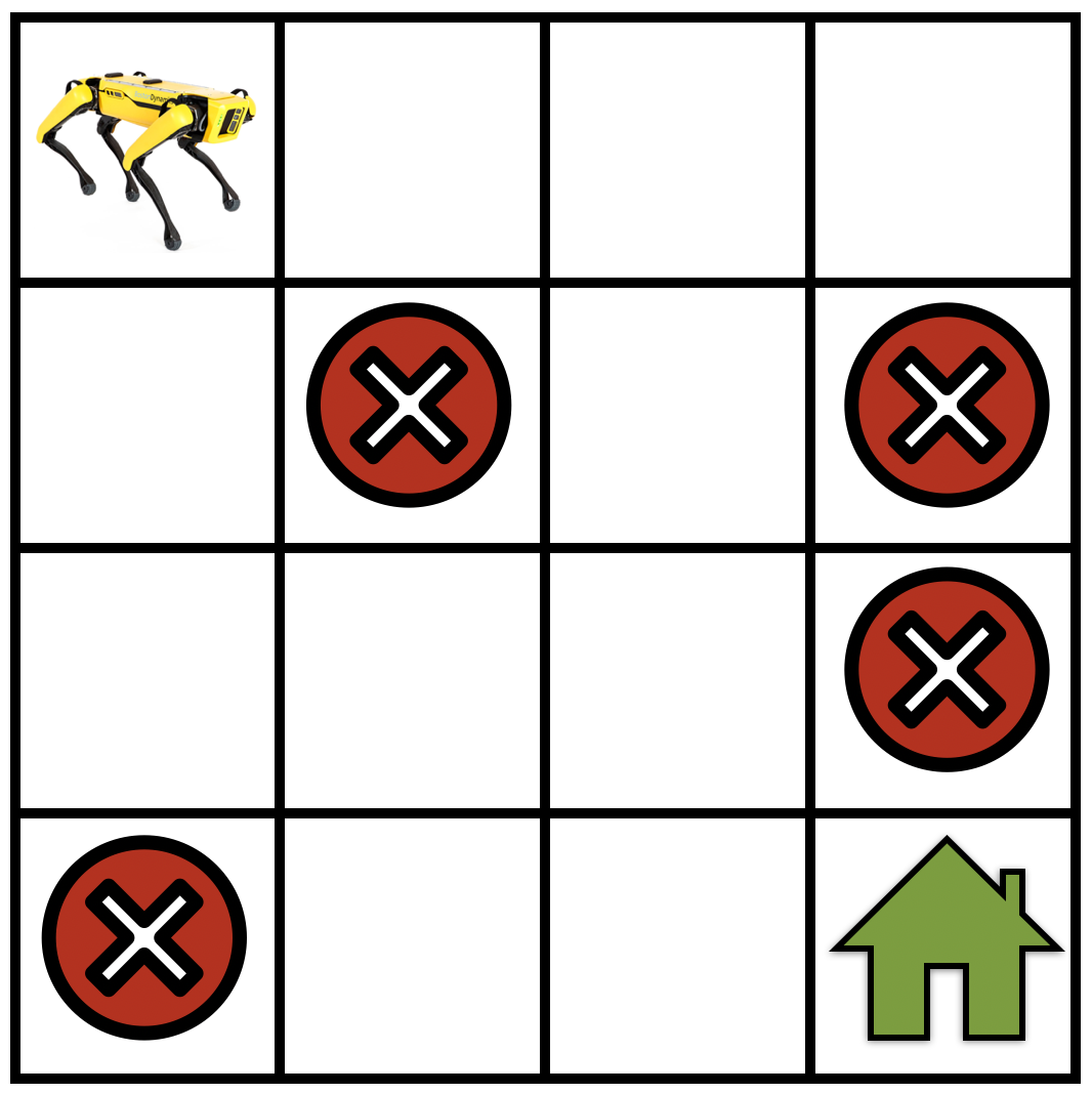
The state space, denoted by $S$, represents all possible configurations or situations the agent can find itself in. Think of it as the comprehensive map of the environment’s “reality” at any given moment. The nature of the state space can vary drastically depending on the problem. In a simple game like Tic-Tac-Toe, the state can be represented by the current arrangement of ‘X’s and ‘O’s on the board. For a robot navigating a maze, a state might be its current coordinates and orientation. In more complex scenarios, such as a stock trading algorithm, a state could be a vector of financial indicators, news sentiment scores, and historical price data.
The size and nature of the state space are crucial. A finite and relatively small state space makes solving an MDP considerably easier. However, many real-world problems involve continuous or astronomically large state spaces, which necessitate approximation techniques and more sophisticated algorithms. The concept of observability is also tied to the state space. In a fully observable MDP, the agent knows its exact state at all times. In contrast, partially observable MDPs (POMDPs) present a more realistic scenario where the agent only receives observations that are probabilistically related to the true underlying state, adding a layer of uncertainty and requiring agents to maintain beliefs about the state.
The Action Space (A)
The action space, denoted by $A$, encompasses all the possible actions that the agent can take in any given state. These are the choices the agent has to influence its environment. Similar to the state space, the action space can be finite or infinite. In the Tic-Tac-Toe example, the actions are placing an ‘X’ or ‘O’ in an empty square. For a robot, actions might include moving forward, turning left, or picking up an object. For a recommendation system, an action could be recommending a specific product or content item to a user.
The action space is typically defined for each state, meaning that not all actions may be available in every state. For instance, an agent cannot place a piece on an already occupied square in Tic-Tac-Toe. The cardinality of the action space significantly impacts the complexity of the learning problem. A larger action space generally leads to a more challenging exploration and learning process.
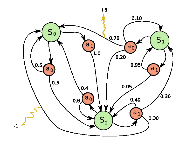
The Transition Probability Function (P)
The transition probability function, often denoted as $P(s’ | s, a)$, is the core of the environment’s dynamics and introduces the element of stochasticity, or randomness, into the MDP. It quantifies the probability of transitioning to a new state $s’$ from the current state $s$ after taking action $a$. This function encapsulates how the environment reacts to the agent’s decisions.
For example, if an agent attempts to move forward in a robot navigation task, $P(s’ | s, text{move forward})$ might indicate the probability of successfully reaching the intended adjacent state $s’$ versus encountering an obstacle and remaining in the same state $s$, or even moving to an unintended state due to slippery surfaces or sensor noise. In a game, this could represent the probability of a certain outcome occurring after a player makes a move, considering factors like opponent actions or random events (e.g., dice rolls in a board game).
A key characteristic of MDPs is the Markov Property. This property states that the future state depends only on the current state and the action taken, and not on the history of states and actions that led to the current state. Mathematically, this means:
$P(s{t+1} | st, at, s{t-1}, a{t-1}, …, s0, a0) = P(s{t+1} | st, at)$
This assumption significantly simplifies the problem by allowing us to disregard the past when making predictions about the future, provided we know the current state.
The Reward Function (R)
The reward function, $R(s, a, s’)$, defines the immediate feedback the agent receives after transitioning from state $s$ to state $s’$ by taking action $a$. This is the crucial signal that guides the agent’s learning. Rewards can be positive (encouraging certain behaviors) or negative (penalizing undesirable behaviors). The ultimate goal of an RL agent is to maximize its cumulative reward over time.
The reward function is designed by the problem setter to reflect the desired objective. In a maze navigation task, reaching the goal might yield a large positive reward, while hitting a wall might incur a small negative reward. In a game, scoring points corresponds to positive rewards, and losing lives to negative rewards. For a financial trading agent, profit would be a positive reward, and losses a negative reward.
The design of an effective reward function is often one of the most challenging aspects of applying RL. A poorly designed reward function can lead to unintended behaviors or an agent that fails to achieve the true objective. For example, an agent tasked with cleaning a room might learn to repeatedly pick up and drop an object if the reward is solely based on the number of times it interacts with objects, rather than on the state of the room being clean.
Discount Factor ($gamma$)
The discount factor, denoted by $gamma$, is a value between 0 and 1 that determines the importance of future rewards relative to immediate rewards. It is a crucial parameter in defining the objective of an RL agent.
- If $gamma = 0$, the agent is myopic and only cares about immediate rewards.
- If $gamma$ is close to 1, the agent is far-sighted and values future rewards highly.
The cumulative reward at time $t$ is typically defined as:
$Gt = R{t+1} + gamma R{t+2} + gamma^2 R{t+3} + … = sum{k=0}^{infty} gamma^k R{t+k+1}$
The discount factor ensures that the sum of rewards converges, especially in infinite-horizon problems. It also intuitively reflects the idea that rewards received sooner are generally more valuable than rewards received later, due to factors like uncertainty about the future or the time value of money.
The Goal of Reinforcement Learning within an MDP: Policies and Value Functions
With the components of an MDP laid out, the next logical step is to understand what an RL agent strives to achieve. The overarching goal is to learn an optimal strategy, or policy, that dictates the agent’s behavior in any given state to maximize its expected cumulative reward.
Policies ($pi$)
A policy, denoted by $pi(a | s)$, is a mapping from states to actions. It defines the agent’s behavior. There are two main types of policies:
- Deterministic Policy: $pi(s) = a$ – For each state $s$, the policy specifies a single action $a$ to take.
- Stochastic Policy: $pi(a | s)$ – For each state $s$, the policy specifies a probability distribution over the available actions. This means the agent might choose different actions in the same state, with probabilities dictated by the policy. Stochastic policies are more general and can be useful for exploration.
The goal of an RL algorithm is to find an optimal policy, denoted by $pi^*$, which yields the highest possible expected cumulative reward from any state.
Value Functions
To determine the “goodness” of a state or a state-action pair, we use value functions. These functions quantify the expected future reward.
- State-Value Function ($V^pi(s)$): This function represents the expected cumulative reward an agent will receive starting from state $s$ and following policy $pi$ thereafter.
$V^pi(s) = Epi [Gt | S_t = s]$
- Action-Value Function ($Q^pi(s, a)$): This function represents the expected cumulative reward an agent will receive starting from state $s$, taking action $a$, and then following policy $pi$ thereafter.
$Q^pi(s, a) = Epi [Gt | St = s, At = a]$
The $Q$-function is particularly important because if an agent knows the optimal $Q$-function, $Q^(s, a)$, it can easily derive the optimal policy: at any state $s$, the agent should choose the action $a$ that maximizes $Q^(s, a)$.
Bellman Equations
The Bellman equations are a set of fundamental equations in RL that describe the relationship between the value of a state (or state-action pair) and the values of its successor states. They are recursive and form the basis for many RL algorithms.
The Bellman Expectation Equation for the state-value function $V^pi(s)$ under policy $pi$ is:
$V^pi(s) = sum{a} pi(a|s) sum{s’} P(s’ | s, a) [R(s, a, s’) + gamma V^pi(s’)]$
And for the action-value function $Q^pi(s, a)$:
$Q^pi(s, a) = sum{s’} P(s’ | s, a) [R(s, a, s’) + gamma sum{a’} pi(a’|s’) Q^pi(s’, a’)]$
These equations highlight that the value of a state/action is the expected immediate reward plus the discounted expected value of the next state/action, averaged over all possible transitions and subsequent actions according to the policy.
The Bellman Optimality Equation defines the value of the optimal policy $pi^*$:
$V^(s) = max{a} sum{s’} P(s’ | s, a) [R(s, a, s’) + gamma V^(s’)]$
$Q^(s, a) = sum{s’} P(s’ | s, a) [R(s, a, s’) + gamma max{a’} Q^(s’, a’)]$
Finding solutions to these Bellman optimality equations is equivalent to finding the optimal policy and its associated value function. Algorithms like Value Iteration and Policy Iteration are designed to converge to these optimal values.
The Power and Applications of MDPs in AI
The theoretical elegance of MDPs is matched by their practical utility across a wide spectrum of AI applications. By providing a formal framework for sequential decision-making, MDPs enable the development of intelligent agents capable of learning and adapting in dynamic environments.
Solving the MDP: Algorithms and Approaches
The process of finding an optimal policy for an MDP is known as “solving the MDP.” Several classes of algorithms exist for this purpose, broadly categorized as:
-
Dynamic Programming: These methods require a complete model of the environment (i.e., knowledge of $P$ and $R$). Algorithms like Value Iteration and Policy Iteration iteratively update value functions until convergence to the optimal values. They are highly efficient when the model is known and the state space is manageable, but less applicable in situations where the environment dynamics are unknown.
-
Monte Carlo Methods: These methods learn from experience by averaging returns over complete episodes. They do not require a model of the environment. They can be used to estimate value functions and improve policies after an episode has concluded.
-
Temporal-Difference (TD) Learning: TD methods combine ideas from Monte Carlo and Dynamic Programming. They learn from incomplete episodes by bootstrapping, meaning they update estimates based on other learned estimates. Algorithms like Q-learning and SARSA are prominent examples of TD methods and are highly effective for learning optimal policies without a model.
-
Deep Reinforcement Learning: When dealing with very large or continuous state and action spaces, traditional methods become intractable. Deep Reinforcement Learning (DRL) combines deep neural networks with RL algorithms. Neural networks are used to approximate value functions or policies, allowing agents to learn from high-dimensional inputs like raw sensory data (e.g., images). This has led to breakthroughs in areas like game playing (e.g., AlphaGo) and robotics.
Real-World Impact and Future Directions
The theoretical foundation of MDPs underpins a vast array of modern AI applications:
- Robotics: Controlling robot arms, autonomous navigation, and multi-robot coordination rely heavily on MDP formulations to optimize movement and task completion.
- Game Playing: From classic board games to complex video games, RL agents trained within MDP frameworks have achieved superhuman performance.
- Recommender Systems: Personalizing product or content recommendations by learning user preferences and predicting future engagement can be framed as an MDP problem.
- Autonomous Vehicles: Decision-making for self-driving cars, such as steering, acceleration, and lane changes, often involves MDP-based control policies.
- Healthcare: Optimizing treatment strategies for chronic diseases or drug discovery processes can be approached using MDPs.
- Finance: Algorithmic trading, portfolio optimization, and risk management are areas where MDPs offer powerful solutions.
As AI continues to advance, the understanding and application of Markov Decision Processes will remain central. Future research will focus on developing more efficient and robust algorithms, handling partial observability more effectively, addressing complex multi-agent scenarios, and ensuring the safety and interpretability of RL systems. The ability to model and solve sequential decision-making problems, as elegantly captured by the MDP framework, is a cornerstone of artificial intelligence, driving innovation and shaping the technological landscape of tomorrow.
aViewFromTheCave is a participant in the Amazon Services LLC Associates Program, an affiliate advertising program designed to provide a means for sites to earn advertising fees by advertising and linking to Amazon.com. Amazon, the Amazon logo, AmazonSupply, and the AmazonSupply logo are trademarks of Amazon.com, Inc. or its affiliates. As an Amazon Associate we earn affiliate commissions from qualifying purchases.