In the vast and evolving landscape of data management, the ability to store, process, and analyze information efficiently is paramount. Businesses today generate an unprecedented volume of data, and extracting meaningful insights from this deluge is a critical competitive advantage. While traditional databases excel at transactional processing, they often fall short when it comes to complex analytical queries necessary for business intelligence. This is where the concept of a “star schema” shines – a cornerstone of data warehousing architecture designed specifically to optimize data retrieval and analysis.
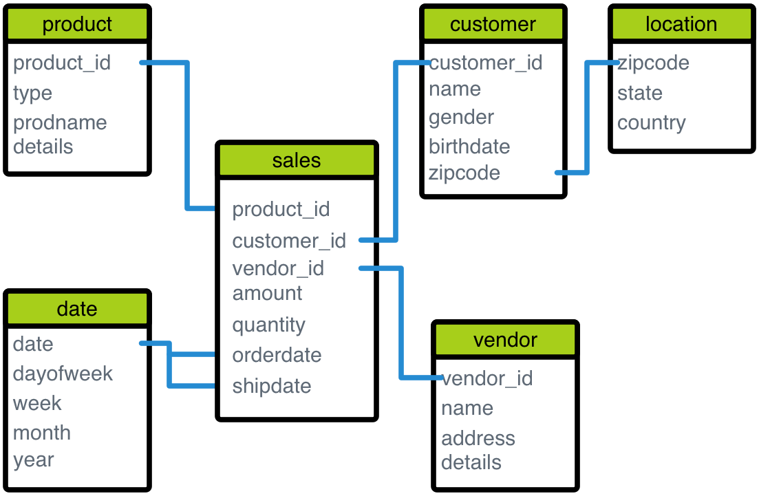
At its core, a star schema is a simplified dimensional model characterized by a central “fact” table connected to multiple “dimension” tables. This structure, which resembles a star with the fact table at the center and dimension tables radiating outwards, is the bedrock for Online Analytical Processing (OLAP) and empowers organizations to perform sophisticated analyses with remarkable speed and clarity. It’s not just a database design; it’s a strategic architectural choice that enables faster decision-making and a deeper understanding of business performance.

The Foundation: Data Warehousing and Analytical Needs
To truly grasp the significance of the star schema, it’s essential to understand the fundamental difference between operational data systems and analytical data systems. These two paradigms serve distinct purposes within an organization, and each demands a unique approach to data modeling.
Transactional vs. Analytical Systems (OLTP vs. OLAP)
Operational systems, often referred to as Online Transaction Processing (OLTP) systems, are the backbone of daily business operations. Think of systems managing sales orders, inventory, banking transactions, or customer registrations. These systems are optimized for frequent, small, and fast read/write operations. Their database schemas are typically highly normalized, meaning data redundancy is minimized by breaking down information into many smaller, linked tables. While normalization ensures data integrity and efficiency for transactional updates, it can make complex analytical queries involving many joins across numerous tables slow and cumbersome.
In contrast, analytical systems, or Online Analytical Processing (OLAP) systems, are designed for querying and reporting on historical data. They are built to answer complex business questions such as “What were our sales trends for product category X in region Y over the last quarter?” or “Which customer segments are most profitable?” OLAP systems prioritize fast data retrieval and aggregation over quick writes. They consolidate vast amounts of historical data, often from multiple source systems, into a single repository known as a data warehouse. This distinction is crucial, as the performance requirements for analytical queries necessitate a departure from the normalized structures of OLTP.
The Role of Data Warehouses
A data warehouse acts as a central repository for integrated, subject-oriented, time-variant, and non-volatile data, making it suitable for analytical reporting and business intelligence. It gathers data from various operational systems, cleanses it, transforms it, and loads it into a structure optimized for analysis. The key characteristic here is “optimized for analysis.” Unlike operational databases, which are designed to support the flow of business transactions, data warehouses are purpose-built to facilitate insightful queries, trend analysis, and strategic decision-making. The star schema is one of the most popular and effective models for structuring data within a data warehouse, precisely because it addresses the limitations of OLTP schemas for analytical workloads.
Deconstructing the Star Schema: Fact and Dimension Tables
The elegance and efficiency of the star schema stem from its straightforward, two-table type structure: the central fact table and its surrounding dimension tables.
The Central Fact Table
At the heart of every star schema lies the fact table. This table contains the quantitative data, or “facts,” that are the subject of analysis. These facts are typically numerical measures that are additive or semi-additive, such as sales quantity, revenue, cost, profit, or transaction count. Each row in a fact table represents a specific event or transaction at a particular level of granularity. For instance, in a sales fact table, each row might represent a single line item in a sales order.
Crucially, the fact table also contains foreign keys that link it to the primary keys of the associated dimension tables. These foreign keys, in combination, form the composite primary key of the fact table, defining the unique context for each measure. The granularity of the fact table is critical; it dictates the lowest level of detail at which data can be analyzed. If a sales fact table stores data at the individual product sale level, you can aggregate it to analyze sales by day, by customer, by product, or any combination thereof.
The Surrounding Dimension Tables
Radiating out from the central fact table are the dimension tables. These tables provide the descriptive context for the numerical facts. They answer the “who, what, where, when, and how” questions related to the facts. Each dimension table represents a particular business aspect or attribute that might be used to filter or categorize the facts.
Common examples of dimension tables include:
- Product Dimension: Contains attributes like product name, category, brand, color, size.
- Customer Dimension: Contains attributes like customer name, address, age group, loyalty status.
- Time Dimension: Contains attributes like day, week, month, quarter, year, holiday indicator.
- Store/Location Dimension: Contains attributes like store name, city, region, demographics.
- Employee/Salesperson Dimension: Contains attributes like employee ID, name, department, role.
Dimension tables are typically denormalized, meaning they contain all relevant descriptive attributes in a single table, even if some attributes could logically be further broken down into separate tables. This denormalization is a deliberate design choice that simplifies queries by reducing the number of joins required to retrieve descriptive information. For example, a “product” dimension might include both the product name and its category, rather than having a separate “product category” table. Each row in a dimension table represents a unique member of that dimension (e.g., a specific product or a specific customer) and has a unique primary key, often a surrogate key, which is a simple integer ID.
The “Star” Analogy
The name “star schema” perfectly describes its visual layout: the fact table sits at the center, like the core of a star, and the dimension tables are directly connected to it, like points radiating outwards. This direct connection, with no intermediate tables between the fact table and its dimensions, is what makes the star schema so powerful for analytical queries. It ensures that queries can quickly join the fact table to any desired dimension table without navigating through multiple levels of foreign key relationships, as might be necessary in a highly normalized schema.
The Luminous Benefits of the Star Schema
The architectural simplicity of the star schema translates directly into profound advantages for data analysis and business intelligence. Its design choices are geared towards maximizing query performance and ease of use.
Simplified Querying and Reporting
One of the most immediate benefits of the star schema is the drastic simplification of SQL queries. Because all dimensions are directly linked to the fact table, analytical queries typically involve only a few joins (one for each dimension needed in the analysis) to retrieve both the measures and their descriptive context. This contrasts sharply with highly normalized schemas, where a single analytical question might require numerous, complex joins across dozens of tables. This simplicity not only makes it easier for data analysts and developers to write queries but also makes it more intuitive for business users employing self-service BI tools. They can easily drag and drop dimensions and measures, confident that the underlying structure is optimized for their requests.
Enhanced Query Performance
The denormalized nature of dimension tables and the direct links to the fact table significantly boost query performance. Fewer joins mean less computational overhead for the database engine. Additionally, dimension tables are typically much smaller than fact tables and static, allowing for efficient caching. When dimensions are joined with the usually massive fact table, the database can leverage highly optimized join algorithms. This structure is also conducive to efficient indexing strategies, particularly bitmap indexes on dimension keys within the fact table, further accelerating query response times for aggregations and filtering. The result is faster report generation and more responsive interactive dashboards, enabling users to explore data without frustrating delays.

Intuitive Data Understanding
The star schema naturally aligns with how business users conceptualize their data. When a business user thinks about “sales by product and region,” they intuitively map “sales” to the fact table and “product” and “region” to dimension tables. This direct mapping makes the data model highly understandable, even for non-technical stakeholders. It fosters a common language between business and technical teams, reducing misinterpretations and making it easier to design effective reports and dashboards that truly answer business questions. The clarity of the model empowers users to quickly grasp the relationships between different data elements.
Scalability and Flexibility
Star schemas are remarkably scalable and flexible. As new data sources emerge or new analytical requirements arise, new dimensions or new measures can often be added with minimal disruption to the existing structure. For instance, if a company decides to track customer demographics more deeply, a new attribute can be added to the customer dimension table without affecting the fact table or other dimensions. Similarly, if a new measure (like “discount amount”) needs to be tracked, it can be added as a new column to the fact table. This modularity allows data warehouses built on star schemas to evolve with the changing needs of the business without requiring extensive re-engineering, protecting the investment in the data infrastructure.
Crafting Your Constellation: Design Principles and Best Practices
Designing an effective star schema requires careful consideration and adherence to certain best practices to ensure optimal performance, usability, and maintainability.
Identifying Business Processes and Granularity
The first step in designing a star schema is to clearly identify the business processes you want to analyze (e.g., sales, inventory, customer service). For each process, determine the specific business event you want to track. Once the event is identified, establish the granularity of the fact table – the lowest level of detail at which data will be stored. This is arguably the most critical design decision. For example, for sales, is it “each line item in a sales order,” “each complete sales transaction,” or “daily summary sales by store”? The chosen granularity will dictate what questions can be answered and what dimensions are relevant. A lower granularity offers more flexibility for analysis but results in a larger fact table.
Defining Facts and Dimensions
With granularity defined, clearly separate your data into facts (measures) and dimensions (descriptive attributes).
- Measures should be quantifiable and typically additive (e.g., quantity, price, revenue, cost). Avoid placing descriptive text or non-numeric IDs in the fact table.
- Dimensions should provide context to these measures. Every attribute that describes a measure (who, what, when, where, why) belongs in a dimension table. Ensure that dimension tables are comprehensive yet concise, containing only attributes relevant for analysis. Resist the urge to include measures within dimension tables or highly transient data that changes with every transaction.
Handling Slowly Changing Dimensions (SCDs)
One common challenge in data warehousing is handling changes to dimensional attributes over time. For example, a customer’s address might change, or a product’s category might be updated. This is where Slowly Changing Dimensions (SCDs) come into play.
- SCD Type 1: Overwrites the old attribute value with the new one. This approach is simple but loses historical data. (e.g., customer address changes, old address is lost).
- SCD Type 2: Creates a new row in the dimension table for each change, preserving the historical version of the attribute. This requires adding “start date,” “end date,” and “current flag” columns to the dimension. This is generally preferred for analytical purposes as it allows analysts to query historical facts with the attributes that were valid at the time of the event. (e.g., customer moves, a new row is added for the new address, linking to new transactions, while old transactions link to the old address).
Understanding and implementing the appropriate SCD type is crucial for maintaining historical accuracy in analytical reports.
Surrogate Keys
Instead of using the natural primary keys from the source operational systems (e.g., ProductID from the transactional database) as primary keys in dimension tables, it is best practice to use surrogate keys. A surrogate key is a simple, non-intelligent, system-generated integer (e.g., an auto-incrementing ID).
- Benefits:
- Independence: Decouples the data warehouse from changes in source system keys.
- Performance: Integer joins are generally faster than joins on multi-column natural keys or string keys.
- SCD Type 2 Support: Essential for implementing SCD Type 2, as a new surrogate key can be assigned to each new version of a dimension member.
- Simplicity: Simplifies ETL processes and database design.
Denormalization vs. Normalization in Practice
While OLTP systems favor normalization for data integrity and write efficiency, data warehouses, and particularly star schemas, embrace denormalization within their dimension tables. This is a deliberate trade-off: we sacrifice some storage efficiency and update simplicity for significantly improved read performance. By including all relevant attributes directly in the dimension table (e.g., product name, category, and brand in a single Product Dimension table), the need for complex joins between multiple descriptive tables is eliminated during query time. The fact table itself remains “normalized” in the sense that it only contains foreign keys and measures, but the dimensions are intentionally denormalized to flatten the hierarchical structure of descriptive data.
Beyond the Star: Star Schema vs. Snowflake Schema
While the star schema is dominant, another related dimensional model, the snowflake schema, is also used in data warehousing. Understanding their differences is key to choosing the right model for specific analytical needs.
Understanding the Snowflake Schema
The snowflake schema is an extension of the star schema where the dimension tables are normalized. This means that a dimension table can have sub-dimension tables that further describe it. For example, in a star schema, a Product Dimension might contain attributes like ProductCategoryName and ProductBrandName. In a snowflake schema, ProductCategory and ProductBrand might be broken out into separate, smaller dimension tables, each with its own primary key, linked to the Product Dimension table. This creates a branching structure, resembling a snowflake, as dimension tables fan out into further dimensions.
Key Differences and Trade-offs
- Complexity: Snowflake schemas are more complex due to the increased number of tables and the need for more joins to retrieve dimension attributes. Star schemas are simpler, with direct links from fact to dimension.
- Storage: Snowflake schemas generally require less storage space because data redundancy within dimension tables is reduced through normalization. Star schemas, with their denormalized dimensions, might use more storage for repetitive descriptive data.
- Query Performance: Star schemas typically offer superior query performance for analytical queries because fewer joins are required. Snowflake schemas, with their multiple levels of dimension joins, can be slower for complex queries, although modern database optimizers can mitigate this to some extent.
- Maintainability: Star schemas are generally easier to understand and maintain due to their flatter structure. Snowflake schemas can be more challenging to manage, especially during ETL processes.
- Data Integrity: Snowflake schemas offer better data integrity due to normalization, as changes to an attribute in a sub-dimension only need to be updated in one place.
When to Choose Which
- Choose Star Schema for the vast majority of data warehousing scenarios. It’s preferred for its simplicity, ease of use, and, most importantly, its exceptional query performance for analytical workloads. If your primary goal is fast, intuitive business intelligence reporting, the star schema is usually the best choice.
- Choose Snowflake Schema in specific situations:
- When dimension tables are very large and have highly hierarchical structures that naturally lend themselves to further normalization (e.g., deeply nested product categories or organizational structures).
- When storage space is an extremely critical constraint, and the reduction in redundancy offered by normalization is vital.
- When dimension data is frequently updated, and normalization helps maintain consistency.
- When the data model needs to closely reflect a highly normalized source system for specific reasons, potentially simplifying some ETL steps.
In practice, a hybrid approach is sometimes adopted, where core dimensions are star-schema-like, and only very complex, large dimensions are ‘snowflaked’ to a limited degree.
Conclusion
The star schema stands as a foundational and enduring pillar of data warehousing and business intelligence architecture. Its elegant simplicity, characterized by a central fact table surrounded by descriptive dimension tables, is not merely an aesthetic choice but a deliberate engineering decision optimized for analytical performance. By streamlining data retrieval and making the underlying data model intuitively understandable, the star schema empowers organizations to unlock the full potential of their historical data.
In an era where data-driven decision-making is no longer a luxury but a necessity, the star schema provides the clarity and speed required to transform raw information into actionable insights. Whether you are building a new data warehouse or optimizing an existing analytical platform, a deep understanding and thoughtful implementation of the star schema remain an indispensable skill for any tech professional engaged in data architecture and business intelligence. It’s a design pattern that continues to shine brightly, illuminating the path to better business understanding.
aViewFromTheCave is a participant in the Amazon Services LLC Associates Program, an affiliate advertising program designed to provide a means for sites to earn advertising fees by advertising and linking to Amazon.com. Amazon, the Amazon logo, AmazonSupply, and the AmazonSupply logo are trademarks of Amazon.com, Inc. or its affiliates. As an Amazon Associate we earn affiliate commissions from qualifying purchases.